Simulation
Random Variate Generation
59 minute read
Notice a tyop typo? Please submit an issue or open a PR.
Random Variate Generation
Inverse Transform Method
In this lesson, we'll go into some additional detail regarding the inverse transform method.
Inverse Transform Method
The inverse transform method states that, if is a continuous random variable with cdf , then . In other words, if we plug a random variable, from any distribution, into its own cdf, we get a Unif(0,1) random variable.
We can prove the inverse transform method. Let . Since is a random variable, it has a cdf, which we can denote . By definition:
Since :
Since is a continuous random variable, its cdf is continuous. Therefore, we can apply the inverse, , to both sides of the inequality:
What is ? Simply, :
Notice that we have an expression of the form ), where . We know, by definition, , so:
In summary, the cdf of is . If we take the derivative of the cdf to get the pdf, we see that . Let's remember the pdf for a uniform random variable:
If , then . Therefore, .
How Do We Use This Result
Let . Since , then . In other words, if we set , and then solve for , we get a random variable from the same distribution as , but in terms of .
Here is how we use the inverse transform method for generating a random variable having cdf : 1. Sample from 2. Return
Illustration
Consider the following cdf, .
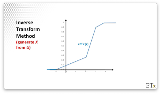
Let's think about the range of . Since we are dealing with a cdf, we know that . Note that, correspondingly, . This means that, for a given Unif(0,1) random variable, , we can generate an , such that , by taking the inverse of with : .
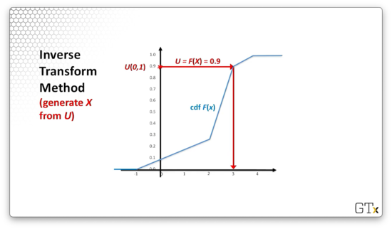
Let's look at an example. Suppose we generate . Let's draw a horizontal line to the graph of . From there, if we draw a vertical line down to the -axis, the -coordinate of the intersection is . In this case, .
Uniform Example
Consider the distribution, which has the following cdf:
Let's set and solve for :
Intuitively, this result makes perfect sense. If we take a Unif(0,1) random variable, and multiply it by , we end up with a Unif(0, ) random variable. Then, if we add to each end, we get a Unif(, ) random variable.
Exponential Example
Consider the distribution, which has the following cdf:
Let's set and solve for :
Also, we know that the expression is itself uniform, so we can simplify:
Inverse Transform Method - Continuous Examples
In this lesson, we'll apply the inverse transform method to trickier continuous examples.
Weibull Example
Let's start with the Weibull distribution, which has the following cdf:
We can solve for :
As we saw before, we know that the expression is itself uniform, so we can simplify:
Notice that, if , . We say that the Weibull distribution generalizes the exponential distribution.
Triangular Example
Now let's look at the triangular distribution. This distribution is important when we don't have a lot of data. For example, suppose we ask someone how long it takes to complete a particular job. Without much data, all they might be able to tell us is the minimum, maximum, and most common (mode) amounts of time. A triangular distribution - parameterized by these three values - is often a good first approximation.
Let's specifically consider the triangular(0,1,2) distribution, which has the following pdf:
If we integrate, we get the following cdf:
Since the cdf contains distinct expressions for different ranges of , we need to transform each expression independently. How do we know which uniforms belong to which expressions? Well, the cdf evaluates the top expression for the first half of the possible -values and the bottom expression for the second half, so we can similarly divide the unit interval in half.
Specifically, if , we solve to get . Note that the square root technically contains both negative and positive roots, but we only consider the positive root since we know that must be between zero and one.
If , we solve the second expression for :
Technically, we could have a in front of the square root, but it doesn't make sense to consider the positive root since must be between one and two. In this case, we only consider the negative root to keep within bounds.
Be aware that we cannot replace with in this example. We need to keep bounded appropriately. For example, suppose we made the replacement and drew . Then, , which doesn't make sense since we know that must be between one and two.
In any event, let's look at two simple examples. If , we evaluate . Alternatively, if , then .
Inverse Transform Method - Continuous Examples - DEMO 1
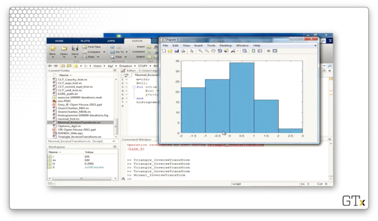
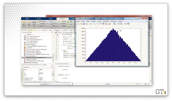
In this demo, we'll look at some Matlab code that applies the inverse transform method to simulate a triangular(0,1,2) random variable. Here's the code.
m = 100;
X = [];
for i=1:m
U = rand;
if U < 0.5
X(i) = sqrt(2 * U);
else
X(i) = 2 - sqrt(2 * (1-U));
end
i = i+1;
end
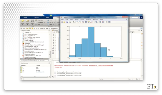
histogram(X)First, we initialize an empty array, X, and then we iterate one hundred times. On each iteration, we sample a uniform random variable with the rand function, perform the appropriate transform depending on whether U < 0.5, and then store the result in X. After we finish iterating, we plot a histogram of the elements in X.
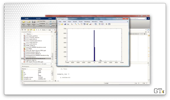
Let's take a look at the histogram we created, which slightly resembles a triangle.
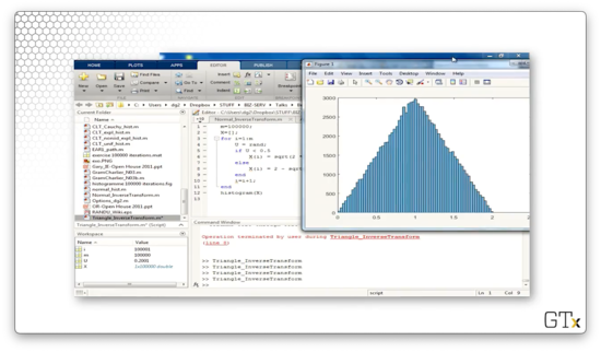
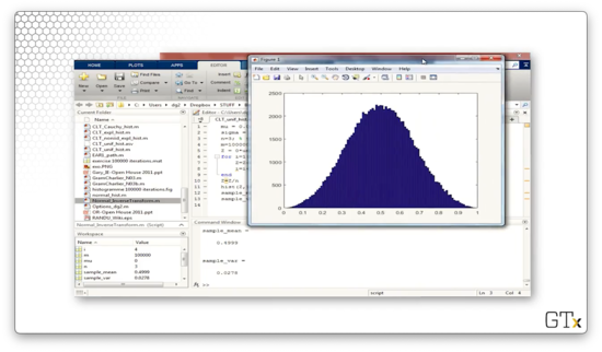
Now, let's iterate one hundred thousand times and look at the resulting histogram. This result looks much nicer.
Inverse Transform Method - Continuous Examples - DEMO 2
Now, let's talk about generating standard normal random variates. Remember our general formula: to compute , we first set and then solve for .
Unfortunately, the inverse cdf of the normal distribution, , does not have an analytical form, which means we can't use our normal approach. This obstacle frequently occurs when working with the inverse transform method.
Generating Standard Normal Random Variables
One easy solution to get around this issue is to look up the values in a standard normal table. For instance, if , then the value of , for which , is . If we want to compute in Excel, we can execute this function: NORMSINV(0.975).
We can also use the following crude approximation for , which gives at least one decimal place of accuracy for :
Here's a more accurate, albeit significantly more complicated, approximation, which has an absolute error :
Transforming Standard Normals to Other Normals
Now, suppose we have , and we want . We can apply the following transformation:
Note that we multiply by , not !
Let's look at an example. Suppose we want to generate , and we start with . We know that:
Remember that :
If we compute , using one of the methods above, we get . Now we can plug and chug:
Matlab Demonstration
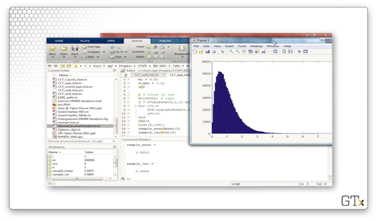
Let's look at some Matlab code to generate standard normal random variables from Unif(0,1) observations. Consider the following:
m = 100;
x = [];
for i=1:m
X(i) = norminv(rand, 0, 1);
i = i + 1;
end
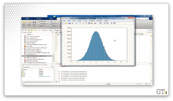
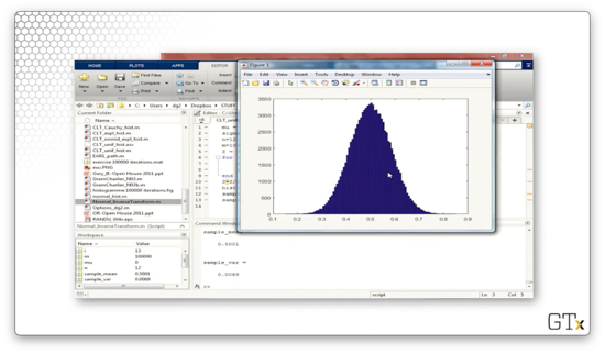
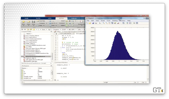
histogram(X)First, we initialize an empty array, X, and then we iterate one hundred times. On each iteration, we first sample a Unif(0,1) random variable with the rand function. Next, we transform it into a Nor(0,1) random variable using the norminv function, which receives a real number, a mean, and a standard deviation and returns the transformed value. Finally, we store the result in X. After we finish iterating, we plot a histogram of the elements in X.
Let's look at the resulting histogram, which doesn't look like the famous bell curve since we are only drawing one hundred observations.
Let's now sample one hundred thousand uniforms and plot the corresponding histogram. This result looks much prettier.
Inverse Transform Method - Discrete Examples
In this lesson, we will use the inverse transform method to generate discrete random variables.
Discrete Examples
It's often best to construct a table for discrete distributions when looking to apply the inverse transform method, especially if the distribution doesn't take on too many values.
Bernoulli Example
Let's look at the Bern() distribution. takes on the value of one with probability and the value zero with probability .
The cdf, , takes on the value for since . For , , since .
Let's construct a table to see how we might map the unit interval onto these two values of :
Since occurs with probability , we transform all uniforms on the range to . This leaves a range of uniforms of width , which map to , from which we draw values with probability .
Here's a simple implementation. If we draw a uniform , then we take ; otherwise, we take . For example, if , and , we take since .
Alternatively, we can construct the following "backwards" table, starting with instead of , which isn't a strict application of the inverse transform method. However, this approach slices the uniforms in a much more intuitive manner. Here's the table:
Here, we take if , which occurs with probability , and we take if , which occurs with probability .
Generic Example
Consider this slightly less-trivial pmf:
Remember that, for a discrete distribution, , where . Correspondingly, the range of uniforms that maps to is bounded by . For example, if , we take .
Discrete Uniform Example
Sometimes, there's an easy way to avoid constructing a table. For example, consider the discrete uniform distribution over , which has the following pmf:
We can think of this random variable as an -sided die toss. How do we transform a Unif(0,1) correctly? If we take a real number between zero and one and multiply it by , we get a real number between zero and . If we round up, we get an integer between one and . For example, if and , then , where is the ceiling/"round up" function.
Geometric Example
Now let's look at the geometric distribution. Intuitively, this distribution represents the number of Bern() trials until the first success. Therefore, the pmf, , represents the probability that the first success occurs on the -th try: failures, with probability , followed by a single success, with probability .
Accordingly, this distribution has the following pmf and cdf:
Let's set and solve for , finding the minimum such that . After some algebra, we see that:
As we've seen in the past, we can also replace with :
For instance, if , and , we obtain:
We can also generate a Geom() random variable by counting Bern() trials until we see a success. Suppose we want to generate . We can generate Bern() random variables until we see a one. For instance, if we generate , then .
More generally, we generate a Geom() random variable by counting the number of trials until , which occurs with probability for each . For example, if , and we draw , , and , then .
Poisson Example
If we have a discrete distribution, like Pois(), which has an infinite number of values, we could write out table entries until the cdf is nearly one, generate a uniform, , and then search the table to find , such that . Consider the following table:
For example, if we generate a uniform in the range , we select .
Let's look at a concrete example, in which we will generate , which has the following pmf:
We can construct the following table:
For example, if , then .
Inverse Transform Method - Empirical Distributions (OPTIONAL)
In this lesson, we will look at how to apply the inverse transform method to unknown, empirical, continuous distributions. Here, we don't know , so we have to approximate it. We will blend continuous and discrete strategies to transform these random variables.
Continuous Empirical Distributions
If we can't find a good theoretical distribution to model a certain random variable, or we don't have enough data, we can use the empirical cdf of the data, :
Each has a probability of being drawn from our unknown continuous distribution. As a result, we can construct a cdf, , where is equal to the number of observations less than or equal to , divided by the total number of observations.
Note that is a step function, which jumps by at every .
Even though is continuous, the Glivenko-Cantelli Lemma states that for all as . As a result, is a good approximation to the true cdf, .
We can use the ARENA functions DISC and CONT to generate random variables from the empirical cdf's of discrete and random distributions, respectively.
To generate these random variables ourselves, let's first define the ordered points , also called order statistics. Note that we wrap the subscripts in parentheses to differentiate them from the order in which they arrived. For example, if , , and , then , , and .
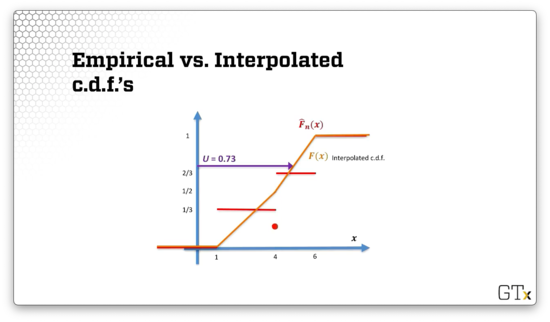
Here's what the empirical cdf looks like, shown in red below:
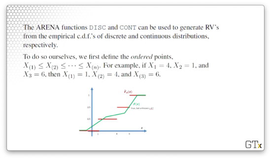
Notice that we step from zero to at , from to at , and to at . If we were to take many observations, then the empirical cdf would approach the true cdf, shown above in green.
Linear Interpolation
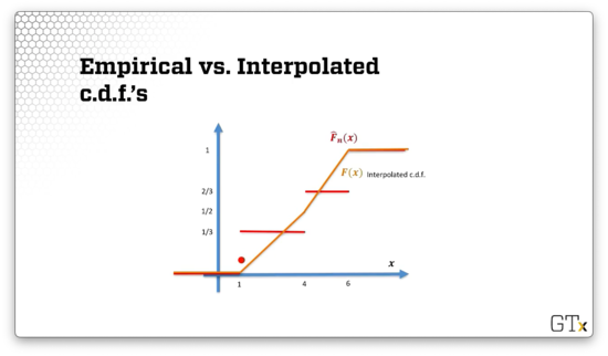
Given that we only have a finite number, , of data points, we can attempt to transform the empirical cdf into a continuous function by using linear interpolation between the 's. Here is the corresponding interpolated cdf (which is not the true cdf even though we denote it as ):
If is less than the first order statistic, then . Given our current observations, we have no evidence that we will encounter a value smaller than our current minimum. Similarly, if is greater than our last order statistic, then . Again, we have no evidence that we will encounter a value greater than our current maximum. For all other points, we interpolate.
Here's the interpolation algorithm. First, we set . Next, we set and . Note that is a discrete uniform random variable over . Finally, we evaluate the following equation for :
Let's break down the above equation. corresponds to our random starting order statistic. The expression turns out to be Unif(0,1): we subtract an integer from the uniform from which it was rounded up and then add one. We multiply that uniform random value by to move the appropriate distance between our starting point and the next order statistic.
For example, suppose , and . If , then and . Then:
Let's see what the linearly interpolated cdf looks like, shown below in orange. Notice that, between and , we have two line segments: one from to , and one from to .
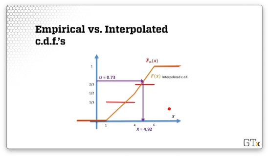
Suppose we draw a uniform, .
If we drop a line from the intersection point with the cdf vertically down, the -coordinate of the intersection with the -axis is .
Alternatively, we can write the interpolated cdf explicitly by using the equation we saw previously and enumerating the two ranges:
If we set and solve for both cases, we have:
Again, if , then .
Convolution Method
In this lesson, we'll look at an alternative to the inverse transform method: the convolution method.
Binomial Example
The term convolution refers to adding things up. For example, if we add up iid Bern() random variables, we get a Binomial(, ) random variable:
We already know how to generate Bern() random variables using the inverse transform method. Suppose we have a collection of uniforms, . If , we set ; otherwise, . If we repeat this process for all and then add up the 's, we get .
For instance, suppose we want to generate . Let's draw three uniforms: , , and . We transform these uniforms into the respective Bern() random variables: , , and . If we add these values together, we get .
Triangular Example
Now let's turn to the Tria(0,1,2) distribution. Remember, we generated triangular random variables using the inverse transform method previously. Alternatively, we can add two iid uniforms together to generate a Tria(0,1,2). In other words, if , then .
Let's look at a pictorial representation of this result.
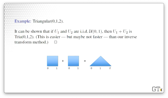
In the Tria(0,1,2) distribution, values close to either end of the range are quite rare. Indeed, it is highly unlikely that two iid uniforms will both have a value very close to zero or one. Values closer to 0.5 are much more likely, and the resulting distribution, which has a maximum probability at , reflects this fact.
This result should remind us of dice toss outcomes. Suppose we toss two six-sided dice. It's highly unlikely for us to see a two or a twelve, each of which occurs with probability , but it's much more common to see a seven, which occurs with probability . There are just more ways to roll a seven.
Erlang Example
Suppose . By definition, the sum of these exponential random variables forms an Erlang() random variable:
Let's use the inverse transform method with convolution to express in terms of uniform random variables. First, let's remember how we transform uniforms into exponential random variables:
Let's rewrite our summation expression to reflect this transformation:
Now, we can take advantage of the fact that and replace natural log invocations with just one. Why might we do this? Natural logarithms are expensive to evaluate on a computer, so we want to reduce them where possible. Consider the following manipulation:
Desert Island Nor(0,1) Approximate Generator
Suppose we have the random variables , and we let equal the summation of the 's: . The central limit theorem tells us that, for large enough , is approximately normal. Furthermore, we know that the mean of is and the variance of is . As a result, .
Let's choose and assume that it's "large enough". Then . If we subtract from , then the resulting mean is , and we end up with a standard normal random variable:
Other Convolution-Related Tidbits
If are iid Geom() random variables, then the sum of the 's is a negative binomial random variable:
If are iid Nor(0, 1) random variables, then sum of the squares of the 's is a random variable:
If are iid Cauchy random variables, then the sample mean, , is also a Cauchy random variable. We might think that is normal for large , but this is not the case as the Cauchy distribution violates the central limit theorem.
Convolution Method DEMO
In this demo, we will look at some of the random variables we can generate using convolution. First, we'll look at how we generate a uniform distribution, which, admittedly, involves no convolution. Consider the following code:
n = 1;
m = 1000000;
Z = 0 * unifrnd(0,1,[1 m]));

for i=1:n
  Z=Z+(unifrnd(0,1,[1 m]));
  i=i+1;
end
Z=Z/n;
hist(Z,100);
This code generates the following histogram, which indeed appears uniform.
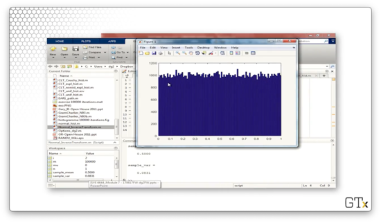
If we change n from one to two, then Z becomes the sum of two uniforms. This code generates the following histogram, which appears triangular, as expected.
Let's change n to three and repeat. The following histogram appears to be taking on a normal shape.
Let's change n to 12 to emulate the "desert island" normal random variable generator we discussed previously. This histogram resembles the normal distribution even more closely.
Now, let's look at generating Exp(1) random variables. Consider the following code:
n = 1;
m = 1000000;
Z = 0 * unifrnd(0,1,[1 m]));

for i=1:n
  Z=Z-log(unifrnd(0,1,[1 m])); % This is the only line that changes
  i=i+1;
end
Z=Z/n;
hist(Z,100);
Here's the corresponding histogram.
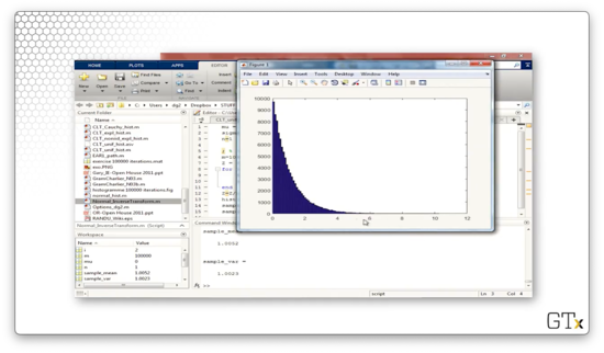
Now, if we change n from one to two, then Z becomes the sum of two exponential random variables, itself an Erlang random variable. Here's the corresponding histogram.
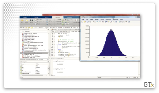
Let's add n=30 exponential random variables, which the central limit theorem tells us will produce an approximately normal result. Here's the histogram. This histogram is clearly not the normal distribution, as it contains considerable right skew.
For a much better approximation, we likely need to add several hundred observations together. Here's the histogram for n=200.
Finally, let's look at generating Cauchy random variables. Consider the following code:
n = 1;
m = 1000;
Z = 0 * unifrnd(0,1,[1 m]));

for i=1:n
  Z=Z + normrnd(0.0, 1.0, [1 m]) ./normrnd(0.0, 1.0, [1 m]) % This is the only line that changes
  i=i+1;
end
Z=Z/n;
hist(Z,100);
If we generate m = 1000 of these random variables, we get the following histogram. The Cauchy distribution has a large variance so, even though most of the observations are close to zero, there are a few observations far out on either side.
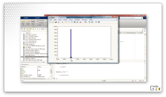
If we add n = 1000 Cauchy random variables, we might expect to see a histogram approximating the normal distribution. However, as we can see from the following plot, the Cauchy distribution violates the central limit theorem.
Acceptance-Rejection Method
In this lesson, we'll talk about the acceptance-rejection method, which is an alternative to the inverse transform method and the convolution technique we studied previously. In contrast to those two methods, acceptance-rejection is very general, and it always works regardless of the random variate we want to generate.
Acceptance-Rejection Method
The motivation for the acceptance-rejection method is that most cdf's cannot be inverted efficiently, which means that the inverse transform method has limited applicability.
The acceptance-rejection method samples from an "easier" distribution, which is close to but not identical to the one we want. Then, it adjusts for this discrepancy by "accepting" (keeping) only a certain proportion of the variates it generates from the approximating distribution.
The acceptance proportion is based on how close the approximate distribution is to the one we want. If the sampling distribution resembles the desired distribution closely, we keep a high proportion of the samples.
Let's look at a simple example. Suppose we want to generate . Of course, we'd usually use the inverse transform method for something so trivial, but let's see how we'd generate using acceptance-rejection.
Here's the algorithm. First, we generate . Next, we check to see if . If so, we accept and set , because the conditional distribution of given that is . If , we reject the observation, and we return to step one, where we draw another uniform. Eventually, we'll get , at which point we stop.
Notation
Suppose we want to simulate a continuous random variable, , with pdf , but is difficult to generate directly. Also suppose that we can easily generate a random variable that has a distinct pdf, , where is a constant and majorizes f(x).
When we say that majorizes , we mean that , for all .
Note that only , not , is a pdf. Since , and the integral of over the real line equals one - by virtue of being a pdf - then the corresponding integral of must be greater than or equal to one. Since doesn't strictly integrate to one, it cannot be a pdf.
Let's look at the constant, . We define , which we assume to be finite, as the integral of over the real line, which we just said was greater than or equal to the corresponding integral of :
Theorem
Let's define a function . We can notice that, since , for all . Additionally, let's sample , and let be a random variable (independent of ), with the pdf we defined earlier: .
If , then the conditional distribution of has pdf . Remember, the random variable we are trying to generate has pdf . In other words, we accept that has the pdf of the random variable we want when .
This result suggests the following acceptance-rejection algorithm for generating a random variable with pdf . First, we generate and with pdf , independent of . If , we accept and we return ; otherwise, we reject and start over, continuing until we produce an acceptable pair. We refer to the event as the acceptance event, which always happens eventually.
Visual Walkthrough
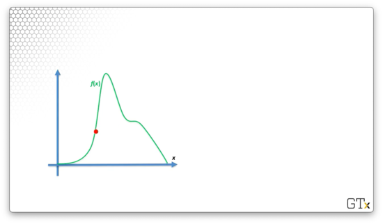
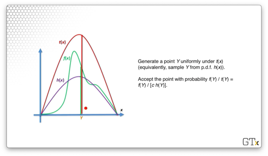
Consider the following pdf, outlined in green, which is the pdf of the random variable we want to generate.
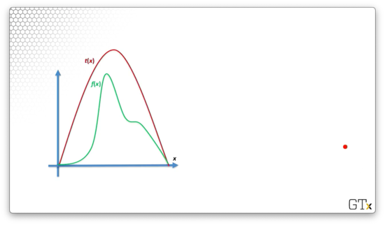
Now consider , shown in red below, which majorizes . As we can see: , for all .
Finally, let's consider , which is defined as , where is the area under . As a result, is proportional to , but has an area equal to one, which makes it a valid pdf.
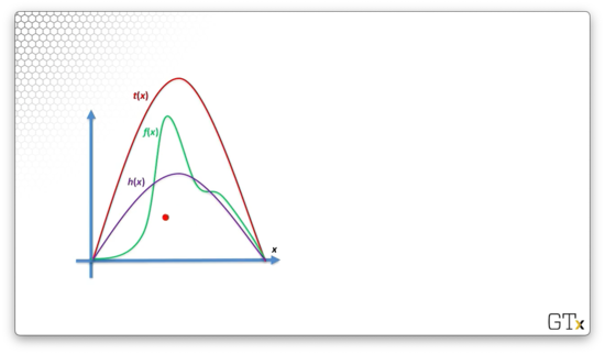
Let's generate a point, , uniformly under . We accept that point with probability . For the point below, we can see the corresponding values of and . As the distance between and decreases, the probability of accepting as a valid value of increases.
Proof of Acceptance-Rejection Method (OPTIONAL)
In this lesson, we will prove the acceptance-rejection method.
A-R Method Recap
Let's define . Remember that is the pdf of the random variable, , that we wish to generate, and majorizes . Let , and let be a random variable, independent of , with pdf .
Note that is not a pdf, but we can transform it into a pdf by dividing it by - the area under - which guarantees that it integrates to one.
If , we set because the conditional distribution of , given , is . Again, we refer to as the acceptance event. We continue sampling and until we have an acceptance, at which point we set and stop.
Proof
We need to prove that the value that comes out of this algorithm, which we claim has pdf , indeed has pdf .
Let be the acceptance event. The cdf of is, by definition:
Given that we have experienced , we have set . As a result, we can express the cdf of with a conditional probability concerning and :
We can expand the conditional probability:
Now, what's the probability of the acceptance event, , given ? Well, from the definition of , we see that:
Since , we can substitute for :
Earlier, we stated that and are independent. As a result, information about gives us no information about , so:
Additionally, we know that is uniform, so, by definition, . Since also has a range of , by definition, then:
Now let's consider the joint probability . Here, we can use the law of total probability, also known as the standard conditioning argument:
We can express directly in the limits of integration, instead of in the conditional probability expression inside the integral. If we integrate over all , such that , then we are still only considering values of such that :
We can substitute :
We might remember, from result above, that . Therefore:
Also remember that, by definition, . Therefore:
If we let , then we have:
Notice that two things changed here. First, we changed the upper limit of integration from to . Second, we changed the probability expression from to . Why? If , , so .
We know that is a pdf, and the integral of a pdf over the real line is equal to one, so:
Together, facts , , and imply that:
Essentially, we have shown that the cdf of is equal to the integral of , from to . If we take the derivative of both sides, we see that the pdf of is equal to .

There are two main issues here. First, we need the ability to sample from quickly since we can't sample from easily. Second, must be small since the probability of the acceptance event is:
Now, is bounded by one from below - - so we want to be as close to one as possible. If so, then:
If , then we accept almost every we sample. If is very large, then is very small, and we will likely have to draw many pairs before acceptance. In fact, the number of trials until "success", defined as , is Geom(), which has an expected value of trials.
A-R Method - Continuous Examples
In this lesson, we will look at some examples of applying the acceptance-rejection method on continuous distributions. As we said, acceptance-rejection is a general method that always works, even when other methods may be difficult to apply.
Theorem Refresher
Define , and note that for all . We sample and from pdf , where majorizes and is the integral of over the real line. If , then has the conditional pdf .
Here's the basic algorithm, which we repeat until acceptance. First, we draw from and from independent of . If , we return . Otherwise, we repeat, sampling and again.
Example
Let's generate a random variable with pdf . This pdf is shown below.
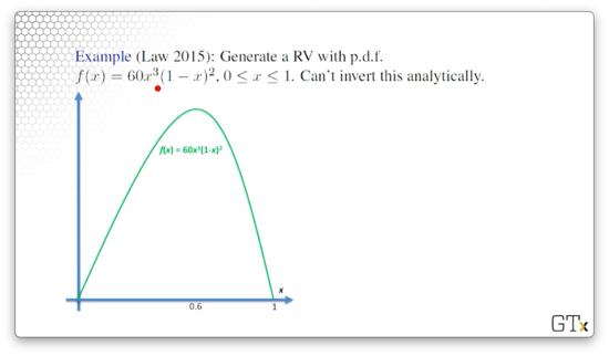
We can't invert this pdf analytically, so we cannot use the inverse transform method; we must use acceptance-rejection. We can use some calculus to determine that the maximum of occurs at : . With this knowledge, we can generate a basic majorizer, .
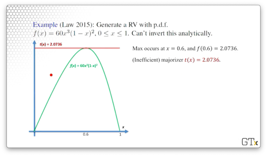
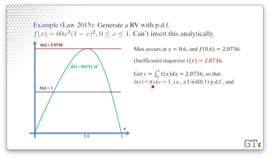
Remember that we said we wanted to be as close to one as possible so that we accept samples from with high probability. We know that equals the integral of from zero to one, so, in this case, . All this to say, is a relatively inefficient majorizer.
Like we said, . In this case, , since . This result means that is a Unif(0,1) random variable, since it's pdf is one.
Finally, let's compute :
Let's look at a simple example. Let's draw two uniforms, and . If we plug and chug, we see that . Therefore, and we take .
A-R Method - Continuous Examples DEMO
Previous Example
Let's demo the acceptance-rejection example we looked at previously. We wanted to generate with pdf . Let's recall :
Additionally, remember that our acceptance event is . Consider the following code:
m = 10000;
X = [];
for i=1:m
U = 1; % Initialize to known failing condition
Y = 0; % Initialize to known failing condition
while U > 60 * (Y^3) * (1-Y)^2 / 2.0736
U = rand;
Y = rand;
end
X(i) = Y;
i=i+1
end
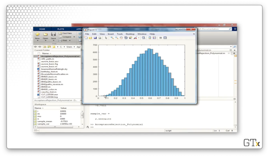
histogram(X)This code iterates for m=10000 iterations and, on each iteration, generates Unif(0,1) random variables, Y and U, until the acceptance event occurs. Once it does, we store away the accepted value of Y and proceed to the next iteration. Finally, we generate a histogram of the m accepted values of Y.
Let's look at the generated histogram after 10,000 samples.
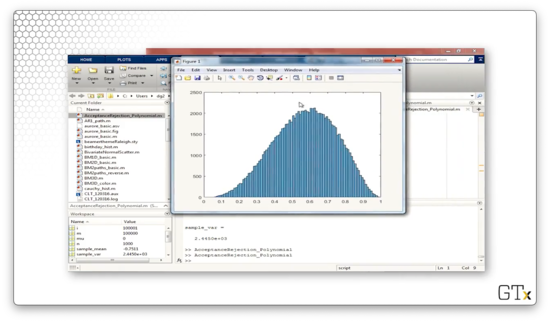
Here's the histogram after 100,000 samples. As we can see, the histogram of generated values looks quite close to the graph of .
Half-Normal Example
In this example, we are going to generate a standard half-normal random variable, which has the following pdf:
This random variable closely resembles a standard normal random variable, except that we've "flipped" the negative portion of the distribution over the -axis and doubled , for all .
We can use the following majorizing function, , as it is always greater than :
If we take the integral of over the domain of , we get :
Now, let's compute :
Let's remember the pdf for an exponential random variable:
We can see that is simply the pdf of an Exp(1) random variable, which we can generate easily!
Finally, let's look at :
To generate a half normal, we simply generate and and accept if .
We can use the half-normal result to generate a Nor(0,1) random variable. We simply have to "flip back" half of the values over the -axis. Given and from the half-normal distribution, we can see that:
As always, we can generate a Nor(, ) by applying the transformation .
A-R Method - Poisson Distribution
In this lesson, we will use a method similar to acceptance-rejection to generate a discrete random variable.
Poisson Distribution
The Poisson distribution has the following pmf:
We'll use a variation of the acceptance-rejection method here to generate a realization of . The algorithm will go through a series of equivalent statements to arrive at a rule that gives for some .
Remember that, by definition, if and only if we observe exactly arrivals from a Poisson() process in one time unit. We can define as the th interarrival time from a Pois() process: the time between arrivals and .
Like we said, if and only if we see exactly Pois() arrivals by . We can express this requirement as an inequality of sums:
In other words, the sum of the first interarrival times must be less than or equal to one, and, correspondingly, the sum of the first interarrival times must be greater than one. Put another way, the th arrival occurs by time , but the th arrival occurs after time .
We might recall that interarrival times from a Pois() are generated from an Exp() distribution, and we know how to transform uniforms into Exp() random variables:
As we saw previously, we can move the natural logarithm outside of the sum and convert the sum to a product: . Consider:
Let's multiply through by - make sure to flip the inequalities when multiplying by a negative - and raise the whole thing by :
To generate a Pois() random variable, we will generate uniforms until the above inequality holds, and then we'll set .
Poisson Generation Algorithm
Let's set , , and . Note that even though we set to , the first thing we do is increment it. As long as , we generate a uniform, . Next, we update our running product, , and we increment by one. Once , we return .
Example
Let's obtain a Pois(2) random variable. We will sample uniforms until the following condition holds:
Consider the following table:
From our iterative sampling above, we see that we take since the inequality above holds for .
Remark
It turns out the the expected number of 's required to generate one realization of is . For example, if , then we need to sample, on average, uniforms before we realize .
This sampling process becomes tedious; thankfully, for large values of , we can take a shortcut. When , then is approximately Nor(, ). We can standardize to get a Nor(0,1) random variable:
Given this fact, we can use the following algorithm to generate a Pois() random variable. First, generate from Nor(0,1). Next, return:
Let's walk through the above expression. The term turns our Nor(0,1) random variable into a Nor(0, ) random variable. If we add , we get a Nor(, ) random variable.
Remember that the normal distribution is continuous, and the Poisson distribution is discrete. We need to discretize our real-valued transformation of , which we accomplish by rounding down. However, if we always round down, then we will underestimate , on average.
We perform a continuity correction by adding before we round, which means that if is between two numbers, we choose the larger number with probability and the lower number with probability .
Finally, we have to take the maximum of our computed value and zero. Why? The standard normal distribution can return negative values, but the Poisson can only return zero or larger.
Let's look at a simple example. If and , then .
Of course, we could have also used the discrete version of the inverse transform method to generate Pois() random variables by tabling the cdf values and mapping them to the appropriate uniform ranges.
OMSCS Notes is made with in NYC by Matt Schlenker.
Copyright © 2019-2023. All rights reserved.
privacy policy