Simulation
Comparing Systems
30 minute read
Notice a tyop typo? Please submit an issue or open a PR.
Comparing Systems
Introduction
Statistics and simulation experiments are typically performed to analyze or compare a small number of systems, say fewer than 200. The exact method of analysis depends on the type of comparison and the properties of the data. For example, we might analyze exponential interarrival data differently than multivariate normal data.
We can use traditional confidence intervals based on the normal or t-distribution - from an introductory statistics class - to analyze one system. If we want to analyze two systems, we could again use confidence intervals for differences.
However, if we want to analyze more than two systems, we need to use more sophisticated ranking and selection approaches.
Confidence Intervals
We can take confidence intervals for:
- means
- variances
- quantiles
- one-sample, two-sample, > two samples
- classical statistics environment (iid normal observations)
- simulation environment (non-iid normal observations)
Confidence Interval for the Mean
In this lesson, we will review and derive the confidence interval for the mean of iid normal data. This review will allow us to move forward and compare two systems.
Confidence Intervals
In the one-sample case, we are interested in obtaining a two-sided confidence interval for the unknown mean, , of a normal distribution.
Suppose we have iid normal data . Further, assume we have an unknown variance, . Given this information, we will use the well-known -distribution based confidence interval.
Let's recall the expression for the sample mean, :
We might remember that the sample mean is itself a normal random variable: .
Recall the expression for the sample variance, :
We might remember that the sample variance is a random variable: .
As it turns out, and are independent. Remember that if , we can standardize with the following transformation:
Let's apply this rule to . Note that we don't know the true variance, , so we have to use . Consider:
Let's divide each side by :
We can see that the expression in the numerator is the standardization of . Let's also substitute in the expression for in the denominator:
Since is the ratio of a normal random variable and a random variable, we know that comes from the -distribution:
This result immediately lets us compute the confidence interval. Let the notation denote the quantile of a -distribution with degrees of freedom. By definition:
Let's substitute in the expression for :
Using some simple algebra, we can express the probability in terms of :
Therefore, we have the following confidence interval for :
Confidence Intervals for the Difference in Two Means
In this lesson, we will compare two systems via two-sample confidence intervals for the difference in two normal means.
Two-Sample Case
Let's suppose that we have two series of observations. The observations are iid normal with mean and variance , and the observations are iid normal with mean and variance .
We have a few techniques at our disposal for producing a confidence interval for the difference between and . We can use the pooled confidence interval method when we assume and are equal but unknown. If both variances are unequal and unknown, we can use the approximate confidence interval method. Finally, we can use a paired confidence interval when we suspect that the 's and 's are correlated.
Pooled Confidence Interval
If the 's and 's are independent but have common, unknown variance, then the usual confidence interval for the difference in the means is:
Here, refers to the pooled variance estimator for , which is a linear combination of the individual sample variances:
Approximate Confidence Interval
If the 's and 's are independent but have uncommon, unknown variance, then the usual confidence interval for the difference in the means is:
Note that we can't use the pooled variance estimator in this case because the variances are different for the 's and the 's.
This confidence interval is not quite exact, since it uses an approximate degrees of freedom, , where:
Example
Let's look at how long it takes two different guys to parallel park two different cars. We will assume all parking times are normal. Consider:
After some algebra, we have the following statistics:
More algebra gives:
We always round down non-integer degrees of freedom since most tables only include integer values, so .
We can plug and chug these values into our expression for the confidence interval. If we want a confidence interval:
Note that this confidence interval includes zero. Informally speaking, the confidence interval is inconclusive regarding which of and is bigger.
Paired Confidence Interval for the Difference in Two Means
In this lesson, we will look at computing confidence intervals for the difference of two means when the observations are correlated. In this case, we use a paired confidence interval.
Paired Confidence Interval
Let's consider two competing normal populations with unknown means, and . Suppose we collect observations from the two populations in pairs. While the different pairs may be independent, it might be the case that the observations in each pair are correlated with one another.
Paired- Setup
For example, let's think of sets of twins in a drug trial. One twin takes a new drug, and the other takes a placebo. We expect that, since the twins are so similar, the difference in their reactions arises solely from the drug's influence.
In other words, we hope to capture the difference between two normal populations more precisely than if we had chosen pairs of random people since this setup eliminates extraneous noise from nature.
We will see this trick again shortly when we use the simulation technique of common random numbers, which involves using the same random numbers as much as possible between competing scenario runs.
Here's our setup. Let's take pairs of observations:
Note that we need to assume that all the 's and 's are jointly normal.
We assume that the variances and are unknown and possibly unequal. Furthermore, we assume that pair is independent of pair , but we cannot assume that, within a pair, is independent of .
We can define the pair-wise differences as the difference between the observations in a pair:
It turns out that the pairwise differences are themselves iid normal with mean and variance , where:
Ideally, we want the covariance between and to be very positive, as this will result in a lower value of . Having a low variance is always good.
Now the problem reduces to the old single-sample case of iid normal observations with unknown mean, , and variance, . Let's calculate the sample mean and sample variance as before:
Just like before, we get the single-sample confidence interval for the difference of the means and :
Example
Let's look at the parallel parking example from the previous lesson, but, in this case, we will have the same person parking both cars. As a result, we expect the times within a pair to be correlated.
By using the same people to park both cars, there will be some correlation between parking times. If we were to compare the differences in this example from those in the previous example, we would notice that we have much more consistent values in this example because we removed the extraneous noise associated with two different individuals.
As we said, the individual people are independent, and the pairs themselves are independent, but the times for the same person to park the two cars are not independent: they are positively correlated.
The two-sided confidence interval is therefore:
The interval is entirely to the left of zero, indicating that : the Cadillac takes longer to park, on average.
This confidence interval is quite a bit shorter - more informative, in other words - than the previous "approximate" two-sample confidence interval, which was . The reason for this difference is that the paired- interval takes advantage of the correlation within observation pairs.
The moral of the story is that we should use the paired- confidence interval when we can.
Confidence Intervals for Mean Differences in Simulations
In this lesson, we will learn how to apply the confidence intervals in a simulation environment where the observations aren't iid normal. The idea here is to use replicate or even batch means as iid normal observations.
Comparison of Simulated Systems
One of the most important uses of simulation output analysis is the comparison of competing systems or alternative system configurations.
For example, we might evaluate two different "restart" strategies that an airline can run following a disrupting snowstorm in the Northeast. We might want to compare the two strategies to see which minimizes a certain cost function associated with the restart.
Simulation is uniquely equipped to help with these types of situations, and many techniques are available. We can use classical confidence intervals adapted to simulations, variance reduction methods, and ranking and selection procedures.
Confidence Intervals for Mean Differences
Let's continue with the airline example we just described. Let represent the cost of the th simulation replication of strategy . Since we are only comparing two strategies, . If we run simulation runs in total then .
We can assume that, within a particular strategy, the replicate means are iid normal with unknown mean and unknown variance, where .
What's the justification for the iid normal assumption? First, we get independent data by controlling the random numbers between replications. We get identically distributed costs between replications by performing them under identical conditions. Finally, we get approximately normal data by adding up (averaging) many sub-costs to get the overall costs for both strategies.
Our goal now is to obtain a confidence interval for the difference in means, .
We will suppose that all the 's are independent of the 's. In other words, scenario one runs are all independent of scenario two runs.
We can define the sample mean, :
We can define the sample variance, :
An approximate confidence interval for the difference of the means is:
Remember the formula for the approximate degrees of freedom, , which we saw earlier:
Suppose that in our airline example, a smaller cost is better - as is usually the case. If the interval lies entirely to the left of zero, then system one is better. If the interval lies entirely to the right of zero, then system two is better. If the interval contains zero, then, statistically, the two systems are about the same.
Alternative Strategy
As an alternative strategy, we can use a confidence interval analogous to the paired- test, especially if we can pair up the two scenarios during each replication.
Specifically, we can take replications from both strategies, and then set difference .
We can take the sample mean and sample variance of the differences:
The paired- confidence interval is very efficient if the correlation between and is greater than zero:
Common Random Numbers
In this lesson, we will start our discussion of variance reduction techniques. We will begin with common random numbers, which are similar to paired- confidence intervals.
Common Random Numbers
The idea behind common random number is the same as that behind a paired- confidence interval. We will use the same pseudo-random numbers in exactly the same ways for corresponding runs of the competing systems.
For example, we might use the same service times or the same interarrival times when simulating different proposed configurations of a particular job shop.
By subjecting the alternative systems to identical experimental conditions, we hope to make it easy to distinguish which system is best even though the respective estimators have sampling error.
Let's consider the case in which we compare two queueing systems, and , based on their expected customer transit times, and . In this case, the smaller -value corresponds to the better system.
Suppose we have estimators, and , for and , respectively. We'll declare that is the better system if . If the two estimators are simulated independently, then the variance of their difference is:
This sum could be very large, and, if it is, our declaration about which system is better might lack conviction. If we could reduce , then we could be much more confident about our declaration. The technique of common random numbers sometimes induces a high positive correlation between the point estimators and .
Since the two estimators are no longer simulated independently, their covariance is greater than zero. Therefore:
Indeed, for any covariance greater than zero:
We can think about this result as a savings in variance. By introducing correlation between the observations, we reduce the variance in the difference of the estimators for the parameter in question.
Demo
In this demo, we will analyze two queueing systems, each with exponential interarrival times and service times, to see which one yields shorter cycle times.
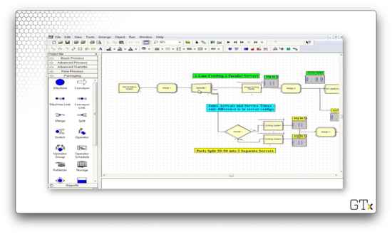
The first strategy involves one line feeding into two parallel servers, and the second strategy involves customers making a 50-50 choice between two lines, each feeding into a single server. We will simulate each alternative for 20 replications of 1000 minutes.
Here's our setup in Arena. On the top, we see one line feeding into two parallel servers. On the bottom, we see the fifty-fifty split between two lines, each feeding into one server.

We might guess that the top scenario is better than the bottom scenario because it might be the case that in the second scenario, we choose to wait in a line even though the other server is free.
In this setup, the arrivals and the service times are generated independently. They are both configured with the same parameters, but the stream of random numbers generated in both systems is distinct.
Let's run the simulation to completion and look at some confidence intervals for the mean cycle time.

For the difference of two means, we get the following confidence interval:
As we expect, this result favors the first system with regard to cycle length.
Now let's look at the same example, but with a slightly different setup.
Here, we generate the arrival times and service times from the same stream of random numbers. Then we duplicate the customers and send each copy to each strategy. We are now simulating the system using common random numbers.
Let's run the simulation to completion and look at some confidence intervals for the mean cycle time.

For the difference of two means, we get the following confidence interval:
As we expect, this result favors the first system with regard to cycle length. What's more, the half-width of the confidence interval is almost one-third that of the setup that didn't use common random numbers.
Antithetic Random Numbers
In this lesson, we will look at the antithetic random numbers method, which intentionally introduces a negative correlation between estimators. This method can be very useful for estimating certain means.
Antithetic Random Numbers
Let's suppose that and are iid unbiased estimators for some parameter . If we can induce a negative correlation between the two estimators, then their average is also unbiased and may have very low variance.
We can express the variance of the average of the two estimators with the following equation:
Since the estimators are identically distributed, , so:
Because we have induced negative correlation, , which means:
Remember that is the usual variance for two iid replications. As we can see, introducing negative correlation results in a variance reduction.
Example
Let's do some Monte Carlo integration using antithetic random numbers to obtain variance reduction. Consider the following integral:
Of course, we know that the true answer of this integral is . Let's use the following Unif(0,1) random numbers, to come up with our usual estimator, , for :
Using the Monte Carlo integration notation from a previous lesson, we have:
Given , , and , we have:
Now, we'll use the following antithetic random numbers, where each here is equal to one minus the corresponding from above:
Then, the antithetic version of the new estimator is:
Again, , , and . If we substitute , we have:
If we take the average of the two answers, we get:
This average is very close to the true answer of 0.693. Using antithetic random numbers, we have introduced a negative correlation between the two estimators and produced an average whose variance is smaller than the average of two iid estimators.
Control Variates
In this lesson, we will look at a final variance reduction technique: control variates. This method is reminiscent of regression methods from an introductory statistics class. This approach takes advantage of knowledge about other random variables related to the one we are interested in simulating.
Control Variates
Suppose our goal is to estimate the mean, , of some simulation output process, . Suppose we somehow know the expected value of some other random variable, . Furthermore, suppose we also know that the covariance between the sample mean, , and is greater than zero.
Obviously, is the usual estimator for , but another estimator for is the so-called control-variate estimator, :
Let's first note the expected value of the control-variate estimator:
Since , we can see that is unbiased for . Now let's take a look at the variance of :
We are hoping that so . Otherwise, we might as well just use by itself.
Now we'd like to minimize with respect to . After some algebra, we see that:
Let's plug in this expression for into our equation for :
Since the second term above is greater than zero, we can see that , which is the result we wanted.
Examples
We might try to estimate a population's mean weight using observed weights with corresponding heights . If we can assume the expected height, , is known, then we can use the control-variate estimator because heights and weights are correlated.
We can also estimate the price of an American stock option, which is tough to estimate, using the corresponding European option price, which is much easier to estimate, as a control.
In any case, many simulation texts give advice on running the simulations of competing systems using common random numbers, antithetic random numbers, and control variates in a useful, efficient way.
Ranking and Selection Methods
In this lesson, we will talk about ranking and selection methods. This lesson aims to give easy-to-use procedures for finding the best system, along with a statistical guarantee that we indeed chose the best system.
Intro to Ranking and Selection
Ranking, selection, and multiple comparison methods form another class of statistical techniques used to compare alternative systems. Here, the experimenter wants to select the best option from a number () of competing processes.
As the experimenter, we specify the desired probability of correctly selecting the best process. We want to get it right, especially if the best process is significantly better than its competitors. These methods are simple to use, somewhat general, and intuitively appealing.
For more than two systems, we could use methods such as simultaneous confidence intervals and ANOVA. However, these methods don't tell us much except that at least one system is different from the others. We want to know specifically which system is best.
What measures might we use to compare different systems? We can ask which system has the biggest mean or the smallest variance. We can ask which treatment has the highest probability of yielding a success or which gives the lowest risk. If we want, we can even select a system based on a combination of criteria.
One example we will look at is determining which of ten fertilizers produces the largest mean crop yield. Another example we will look at involves finding the pain reliever with the highest probability of giving relief for a cough. As a final example, we will determine the most popular former New England football player.
Ranking and selection methods select the best system, or a subset of systems that includes the best, guaranteeing a probability of correct selection that we specify.
Ranking and selection methods are relevant in simulation:
- Normally distributed data by batching
- Independence by controlling random numbers
- Multiple-stage sampling by retaining the seeds
OMSCS Notes is made with in NYC by Matt Schlenker.
Copyright © 2019-2023. All rights reserved.
privacy policy