Simulation
Random Variate Generation, Continued
63 minute read
Notice a tyop typo? Please submit an issue or open a PR.
Random Variate Generation, Continued
Composition (OPTIONAL)
In this lesson, we will learn about the composition method. This technique only works for random variables that are themselves combinations or mixtures of random variables, but it works well when we can use it.
Composition
We use composition when working with a random variable that comes from a combination of two random variables and can be decomposed into its constituent parts.
Let's consider a concrete example. An airplane might be late leaving the gate for two reasons, air traffic delays and maintenance delays, and these two delays compose the overall delay time. Most of the time, the total delay is due to a small air traffic delay, while, less often, the total delay is due to a larger maintenance delay.
If we can break down the total delay into the component delays - air traffic and maintenance - and those components are easy to generate, we can produce an expression for the total delay that combines the individual pieces.
The goal is to generate a random variable with a cdf, , of the following form:
In plain English, we want to generate a random variable whose cdf is a linear combination of other, "easier" cdf's, the 's. Note that and the sum of all 's equals one.
Again, the main idea here is that, instead of trying to generate one complicated random variable, we can generate a collection of simpler random variables, weight them accordingly, and then sum them to realize the single random variable.
Don't fixate on the upper limit being infinity in the summation expression. Infinity is just the theoretical upper limit. In our airplane example, the actual limit was 2.
Here's the algorithm that we will use. First, we generate a positive integer such that for all . Then, we return from cdf .
Proof
Let's look at a proof that has cdf . First, we know that the cdf of , by definition, is . Additionally, by the law of total probability:
Now, we expressed as , and we know that is equal to . Therefore:
Example
Consider the Laplace distribution, with the following pdf and cdf:
Note that the pdf and cdf look similar to those for exponential random variables, except that is allowed to be less than zero and the exponential has a coefficient of one-half. We can think of this distribution as the exponential distribution reflected off the -axis.
Let's decompose this into a "negative exponential" and regular exponential distributions:
If we multiply each CDF here by one-half and sum them together, we get a Laplace random variable:
Let's look at both cases. When :
When :
As we can see, the composed cdf matches the expected cdf, both for and .
The cdf tells us that we generate from half the time and from the other half of the time. Correspondingly, we'll use inverse transform to solve for half the time and we'll solve for the other half. Consider:
Precisely, we transform our uniform into an exponential with probability one-half and a negative exponential with probability negative one-half.
Box-Muller Normal RVs
In this lesson, we will talk about the Box-Muller method, which is a special-case algorithm used to generate standard normal random variables.
Box-Muller Method
If are iid , then the following quantities are iid Nor(0,1):
Note that we must perform the trig calculations in radians! In degrees, is a very small quantity, and resulting and will not be iid Nor(0,1).
Interesting Corollaries
We've mentioned before that if we square a standard normal random variable, we get a chi-squared random variable with one degree of freedom. If we add chi-squared randoms, we get a chi-squared with degrees of freedom:
Meanwhile, let's consider the sum of and algebraically:
Remember from trig class the , so:
Remember also how we transform exponential random variables:
All this to say, we just demonstrated that . Furthermore, and more interestingly, we just proved that:
Let's look at another example. Suppose we take . One standard normal divided by another is a Cauchy random variable, and also a t(1) random variable.
As an aside, we can see how Cauchy random variables take on such a wide range of values. Suppose the normal in the denominator is very close to zero, and the normal in the numerator is further from zero. In that case, the quotient can take on very large positive and negative values.
Moreover:
Thus, we've just proven that . Likewise, we can take , which proves additionally that .
Furthermore:
Polar Method
We can also use the polar method to generate standard normals, and this method is slightly faster than Box-Muller.
First, we generate two uniforms, . Next, let's perform the following transformation:
Finally, we use the acceptance-rejection method. If , we reject and return to sampling uniforms. Otherwise:
We accept . As it turns out, and are iid Nor(0,1). This method is slightly faster than Box-Muller because it avoids expensive trigonometric calculations.
Order Statistics and Other Stuff
In this lesson, we will talk about how to generate order statistics efficiently.
Order Statistics
Suppose that we have the iid observations, from some distribution with cdf . We are interested in generating a random variable, , such that is the minimum of the 's: . Since is itself a random variable, let's call its cdf . Furthermore, since refers to the smallest , it's called the first order statistic.
To generate , we could generate 's individually, which takes units of work. Could we generate more efficiently, using just one ?
The answer is yes! Since the 's are iid, we have:
In English, the cdf of is , which is equivalent to the complement: . Since , .
Now, since the minimum is greater than , then all of the 's must be greater than :
Since the 's are iid, . Therefore:
Finally, note that . Therefore, , so:
At this point, we can use inverse transform to express in terms of :
Example
Suppose . Then:
So, . If we apply inverse transform we get:
We can do the same kind of thing for . Let's try it! If , then we can express as:
Now, since the maximum is less than or equal to , then all of the 's must less than or equal to :
Since the 's are iid, . Therefore:
Finally, note that . Therefore:
Suppose . Then:
Let's apply inverse transform:
Other Stuff
If are iid Nor(0,1), then the sum of the squares of the 's is a chi-squared random variable with degrees of freedom:
If , and , and and are independent, then:
Note that t(1) is the Cauchy distribution.
If , and , and and are independent, then:
If we want to generate random variables from continuous empirical distributions, we'll have to settle for the CONT function in Arena for now.
Multivariate Normal Distribution
In this lesson, we will look at the multivariate normal distribution. This distribution is very important, and people use it all the time to model observations that are correlated with one another.
Bivariate Normal Distribution
Consider a random vector . For example, we might draw from a distribution of heights and from a distribution of weights. This vector has the bivariate normal distribution with means and , variances and , and correlation if it has the following joint pdf:
Note the following definitions for and , which are standardized versions of the corresponding variables:
Let's contrast this pdf with the univariate normal pdf:
The fractions in front of the exponential looks similar in both cases. In fact, we could argue that the fraction for the univariate case might look like this:
In this case, however, , so the expression involving reduces to one. All this to say, the bivariate case expands on the univariate case by incorporating another term. Consider:
Now let's look at the expression inside the exponential. Consider again the exponential for the univariate case:
Again, we might argue that this expression contains a hidden term concerning that gets removed because the correlation of with itself is one:
If we look at the bivariate case again, we see something that looks similar. We retain the coefficient and we square standardized versions of and , although the standardization part is hidden away in and :
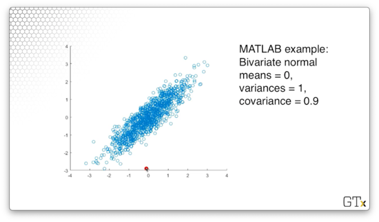
As we said, we can model heights and weights of people as a bivariate normal random variable because those two observations are correlated with one another. In layman's terms: shorter people tend to be lighter, and taller people tend to be heavier.
For example, consider the following observations, taken from a bivariate normal distribution where both means are zero, both variances are one, and the correlation between the two variables is 0.9.
Multivariate Normal
The random vector has the multivariate normal distribution with mean vector and covariance matrix , if it has the following pdf:
Notice that the vector and the vector have the same dimensions: random variable has the expected value .
Now let's talk about the covariance matrix . This matrix has rows and columns, and the cell at the th row and th column holds the covariance between and . Of course, the cell at holds the covariance of with itself, which is just the variance of .
Now let's look at the fraction in front of the exponential expression. Remember that, in one dimension, we took . In dimensions, we take . In one dimension, we take . In dimensions, we take the square root of the determinant of , where the determinant is a generalization of the variance.
Now let's look at the exponential expression. In one dimension, we computed:
In dimensions, we compute:
Here, corresponds to , and is the inverse of the covariance matrix, which corresponds to in the univariate case.
All this to say, the multivariate normal distribution generalizes the univariate normal distribution.
The multivariate case has the following properties:
We can express a random variable coming from this distribution with the following notation: .
Generating Multivariate Random Variables
To generate , let's start out with a vector of iid Nor(0,1) random variables in the same dimension as : . We can express as , where is a -dimensional vector of zeroes and is the identity matrix. Note that the identity matrix makes sense here: since the values are iid, everywhere but the diagonal is zero.
Now, suppose that we can find the lower triangular Cholesky matrix , such that . We can think of this matrix, informally, as the "square root" of the covariance matrix.
It can be shown that is multivariate normal with mean and covariance matrix:
How do we find this magic matrix ? For , we can easily derive :
Again, if we multiply by , we get the covariance matrix, :
Here's how we generate . Since , if we carry the vector addition and matrix multiplication out, we have:
Here's the algorithm for computing a -dimensional Cholesky matrix, .
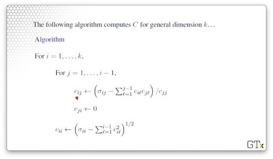
Once we compute , we can easily generate the multivariate normal random variable . First, we generate iid Nor(0,1) uniforms, . Next, we set equal to the following expression:
Note that the sum we take above is nothing more than the sum of the standard normals multiplied by the th row in .
Finally, we return .
Baby Stochastic Processes (OPTIONAL)
In this lesson, we will talk about how we generate some easy stochastic processes: Markov chains and Poisson arrivals.
Markov Chains
A time series is a collection of observations ordered by time: day to day or minute to minute, for instance. We will look at a time series of daily weather observations and determine the probability of moving between two different states, sunny and rainy.
It could be the case that the days are not independent of one another; in other words, if we have thunderstorms today, there is likely a higher than average probability that we will have thunderstorms tomorrow.
Suppose it turns out the probability that we have a thunderstorm tomorrow only depends on whether we had a thunderstorm today, and nothing else. In that case, the sequence of weather outcomes is a type of stochastic process called a Markov chain.
Example
Let's let if it rains on day ; otherwise, . Note that we aren't dealing with Bernoulli observations here because the trials are not independent; that is, the weather on day depends on the weather on day .
We can denote the day-to-day transition probabilities with the following equation:
In other words, refers to the probability of experiencing state on day , given that we experienced state on day . For example, refers to the probability that it is sunny tomorrow, given that it rained today.
Suppose that we know the various transition probabilities, and we have the following probability state matrix:
Remember that state zero is rain and state one is sun. Therefore, means that the probability that we have rain on day given that we had rain on day equals 0.7. Likewise, means that the probability that we have sun on day given that we had rain on day equals 0.3.
Notice that the probabilities add up to one across the rows, signifying that, for a given state on day , the probability of moving to some state on day is one: the process must transition to a new state (of course, this new state could be equivalent to the current state).
Suppose it rains on Monday, and we want to simulate the rest of the week. We will fill out the following table:
Let's talk about the columns. Obviously, the first column refers to the day of the week. The column titled refers to the probability of rain given yesterday's weather. Note that we also represent this probability with , where the dot refers to yesterday's state.
In the third column, we sample a uniform. In the fourth column, we check whether that uniform is less than the transition probability from yesterday's state to rain. Finally, in the fifth column, we remark whether it rains, based on whether the uniform is less than or equal to the transition probability.
Let's see what happens on Tuesday:
Here, we are looking at the probability of transitioning from a rainy day to another rainy day. If we look up that particular probability in our state transition matrix, we get . Next, we sample a uniform, , and check whether that uniform is less than the transition probability. Since , we say that it will rain on Tuesday.
Let's see what happens on Wednesday:
Similarly, we are looking at the probability of again transitioning from a rainy day to another rainy day, so our transition probability is still . We draw another uniform, , and, since , we say that it will rain on Wednesday.
Let's see what happens on Thursday:
Here, we have the same transition probability as previously, but our uniform, , happens to be larger than our transition probability: . As a result, we say that it will not rain on Thursday.
Finally, let's look at Friday:
On Friday, we have a new transition probability. This time, we are looking at the probability of rain given sun, and . Again we draw our uniform, which happens to be greater than the transition probability, so we say it will be sunny on Friday.
Poisson Arrivals
Let's suppose we have a Poisson() process with a constant arrival rate of . The interarrival times of such a process are iid Exp(). Remember that, even though the rate is constant, the arrivals themselves are still random because the interarrival times are random.
Let's look at how we generate the arrival times. Note that we set to initialize the process at time zero. From there, we can compute the th arrival time, , as:
In other words, the next arrival time equals the previous arrival time, plus an exponential random variable referring to the interarrival time. Even more basically, the time at which the next person shows up is equal to the time at which the last person showed up, plus some randomly generated interarrival time.
Note that, even though we seem to be subtracting from , the natural log of is a negative number, so we are, in fact, adding two positive quantities here.
We refer to this iterative process as bootstrapping, whereby we build subsequent arrivals on previous arrivals.
Fixed Arrivals
Suppose we want to generate a fixed number, , arrivals from a Poisson() process in a fixed time interval . Of course, we cannot guarantee any number of arrivals in a fixed time interval in a Poisson process because the interarrival times are random.
It turns out that there is a theorem that states the following: the joint distribution of arrivals from the Poisson process during some interval is equivalent to the joint distribution of the order statistics of iid random variables.
Here's the algorithm. First, we generate iid uniforms, . Next, we sort them: . Finally, we transform them to lie on the interval :
Nonhomogeneous Poisson Processes
In this lesson, we will look at nonhomogeneous Poisson processes (NHPPs), where the arrival rate changes over time. We have to be careful here: we can't use the algorithm we discussed last time to generate arrivals from NHPPs.
NHPPs - Nonstationary Arrivals
An NHPP maintains the same assumptions as a standard Poisson process, except that the arrival rate, , isn't constant, so the stationary increments assumption no longer applies.
Let's define the function , which describes the arrival rate at time . Let's also define the function , which counts the number of arrivals during .
Consider the following theorem to describe the number of arrivals from an NHPP between time and time :
Example
Suppose that the arrival pattern to the Waffle House over a certain time period is an NHPP with . Let's find the probability that there will be exactly four arrivals between times and .
From the equation above, we can see that the number of arrivals in this time interval is:
Since the number of arrivals is , we can calculate the using the pmf, :
Incorrect NHPP Algorithm
Now, let's look at an incorrect algorithm for generating NHPP arrivals. This algorithm is particularly bad because it can "skip" intervals if grows very quickly.
Here's the algorithm.
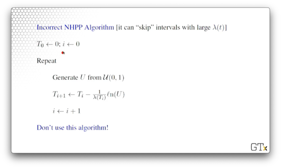
We initialize the algorithm with . To generate the th arrival, we first sample , and then we perform the following computation:
Note that, instead of multiplying by , we multiply by , which is the arrival rate at the time of the previous arrival. The problem arises when the arrival rate radically changes between the time we generate the new arrival and the time that arrival occurs.
Specifically, if , then the arrival rate we use to generate arrival , evaluated at time , is too small. Since we capture the arrival rate of the next arrival at the time of the current arrival, we essentially consider the rate to be fixed between that time and the time the arrival actually occurs.
Thinning Algorithm
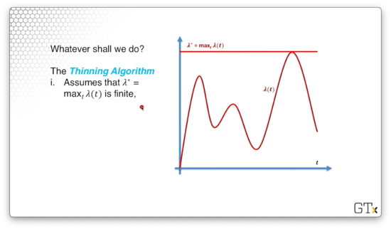
Consider the following rate function, , graphed below. We can suppose, perhaps, that this function depicts the arrivals in a restaurant, and the peaks correspond to breakfast, lunch, and dinner rushes.
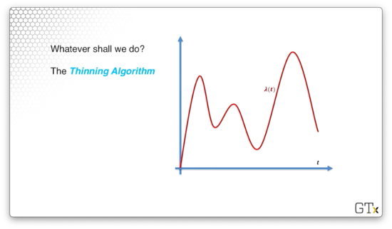
We are going to use the thinning algorithm to generate the th arrival. First, we assume that is finite. We can see the line drawn below.
From there, we will generate potential arrivals at that maximum rate :
We can see the potential arrivals in dotted purple below.
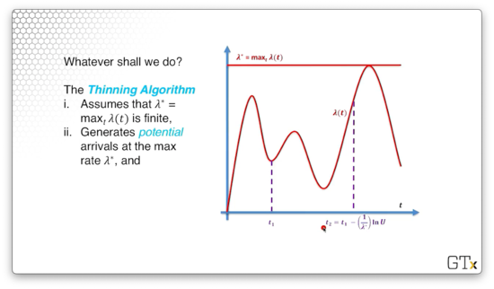
We will accept a potential arrival at time as a real arrival with probability . Thus, as approaches , the likelihood that we accept as a real arrival increases proportionally to . We call this algorithm the thinning algorithm because it thins out potential arrivals.
Let's look at the algorithm.
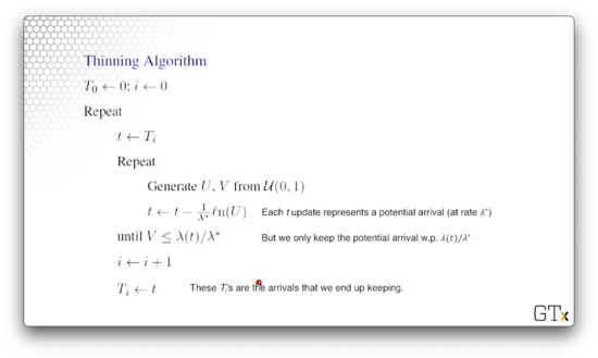
We initialize the algorithm . Next, we initialize , and then we iterate. We generate two iid Unif(0,1) random variables, and , and then we generate a potential arrival:
We keep generating and until this condition holds:
In other words, we only keep the potential arrival with probability . After we accept , we set to , and to , and repeat.
DEMO
In this demo, we will look at how to implement an NHPP in Excel.
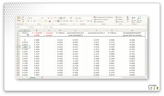
In column A, we have potential NHPP arrival times.
In column B, we have the rate function . Because the sine function is periodic, so are the arrival rates generated by . In fact, never goes below zero, and never goes above two, so .
In column D, we have a sequence of random variables, which we will use to generate interarrival times.
In column E, we generate the potential interarrival times by transforming into an Exp() random variable.
In column F, we bootstrap the arrivals, generating the th arrival by adding the th arrival and the th interarrival time. Note that these potential arrivals are the same values in column A.
In column G, we generate another sequence of random variables , which we will use to determine whether we accept the potential arrival as a real arrival.
In column H, we generate , which refers to the probability that we accept the corresponding potential arrival at time .
If , then we accept the arrival, and we show this boolean value in column I.
In column J, we copy over the real arrival times for all potential arrivals where . Otherwise, we mark the cell as "FALSE".
Finally, in column K, we update the arrival rate for the next iteration.
Here's what the plot of arrival rates over time looks like for this NHPP. Every dot represents an accepted arrival. In the space between the dots, we may have generated potential arrivals, but we didn't accept them as real.
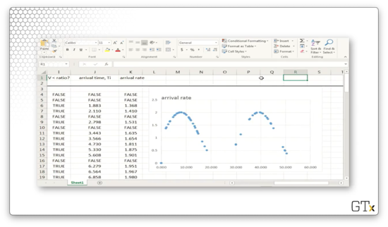
We can see that we have many real arrivals when the is close to and few real arrivals when the two values diverge. Of course, this observation makes sense, given that we accept potential arrivals with probability .
Time Series (OPTIONAL)
In this lesson, we will look at various time series processes, most of which are used in forecasting. In particular, we will be looking at auto-regressive moving average processes (ARMA), which have standard-normal noise, and auto-regressive Pareto (ARP) processes, which have Pareto noise.
First-Order Moving Average Process
A first-order moving average process, or MA(1), is a popular time series for modeling and detecting trends. This process is defined as follows:
Here, is a constant, and the terms are typically iid Nor(0,1) - in practice, they can be iid anything - and they are independent of .
Notice that , and . Both and contain an term; generally, and pairs are correlated.
Let's derive the variance of . Remember, that:
Let's consider :
Now, we know that successive 's are independent, so the covariance is zero:
Furthermore, we know that , so:
Finally, since the 's are Nor(0,1), they both have variance one, leaving us with:
Now, let's look at the covariance between successive pairs. Here's a covariance property:
So:
Since the 's are independent, we know that . So:
We also know that , and, since , . So:
We can also demonstrate, using the above formula, that .
As we can see, the covariances die off pretty quickly. We probably wouldn't use an MA(1) process to model, say month-to-month unemployment, because the unemployment rate among three months is correlated, and this type of process cannot express that.
How might we generate an MA(1) process? Let's start with . Then, we generate to get , to get , and so on. Every time we generate a new , we can compute the corresponding .
First-Order Autoregressive Process
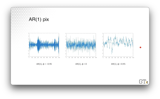
Now let's look at a first-order autoregressive process, or AR(1), which is used to model many different real-world processes. The AR(1) process is defined as:
In order for this process to remain stationary, we need to ensure that , , and that the 's are iid .
Unlike the MA(1) process, non-consecutive observations in the AR(1) process have non-zero correlation. Specifically, the covariance function between and is as follows:
The correlations start out large for consecutive observations and decrease as increases, but they never quite become zero; there is always some correlation between any two observations in the series.
If is close to one, observations in the series are highly positively correlated. Alternatively, if is close to zero, observations in the series are highly negatively correlated. If is close to zero, then the 's are nearly independent.
How do we generate observations from an AR(1) process? Let's start with and to get . Then, we can generate to get , and so on.
Remember that:
So:
Here are the plots of three AR(1) processes, each parameterized with a different value of .
ARMA(p,q) Process
The ARMA(,) process is an obvious generalization of the MA(1) and AR(1) processes, which consists of a th order AR process and a th order MA process, which we will define as:
In the first sum, we can see the autoregressive components, and, in the second sum, we can see the moving average components.
We have to take care to choose the 's and the 's in such a way to ensure that the process doesn't blow up. In any event, ARMA(, ) processes are used in a variety of forecasting and modeling applications.
Exponential AR Process
An exponential autoregressive process, or EAR, is an autoregressive process that has exponential, not normal, noise. Here's the definition:
Here we need to ensure that , , and the 's are iid Exp(1) random variables.
Believe it or not, the EAR(1) has the same covariance function as the AR(1), except that the bounds of are different:
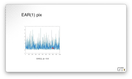
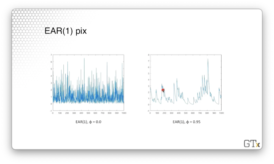
Let's look at a plot of an EAR(1) process with . These observations are iid exponential, and if we were to make a histogram of these observations, it would resemble the exponential distribution.
Here's a plot of an EAR(1) process with . We can see that when successive observations decrease, they appear to decrease exponentially. With probability , they receive a jump from , which causes the graph to shoot up.
Autoregressive Pareto - ARP
A random variable has the Pareto distribution with parameters and if it has the cdf:
This distribution has a very fat tail. In other words, its pdf approaches zero (its cdf approaches one) much more slowly than the normal distribution.
To obtain the ARP process, let's first start off with a regular AR(1) process with normal noise:
Recall that we need to ensure that , , and that the 's are iid . Note that that 's are marginally Nor(0,1), but they are correlated on the order of .
Since the 's are standard normal random variables, we can plug them into their own cdf, to obtain Unif(0,1) random variables: . Since the 's are correlated, so are the 's.
Now, we can feed the correlated 's into the inverse of the Pareto cdf to obtain correlated Pareto observations:
DEMO
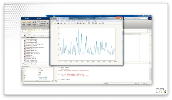
In this demo, we will implement an EAR(1) process in Matlab. Consider the following code:
phi = 0.0;
m = 100;
X = [];
X(1) = exprnd(1,1);
for i=2:m
  X(i) = phi*X(i-1) + (exprnd(1,1) * binornd(1,1-phi));
  i = i+1;
end
Y = [1:m];
plot(Y,X,Y,3,Y,-1)
We start out with phi equal to zero, so we are generating simple exponential observations. We initialize X(1) to exprnd(1,1), which is one Exp(1) observation. Then we iterate.
On each iteration, we set subsequent X(i) entries to phi*X(i-1) + (exprnd(1,1) * binornd(1,1-phi)). Notice the second term in this expression. This term represents adding exponential noise with probability phi. The binornd function returns zero with probability phi, zeroing out the noise, and returns one with probability 1-phi.
Let's see the plot.
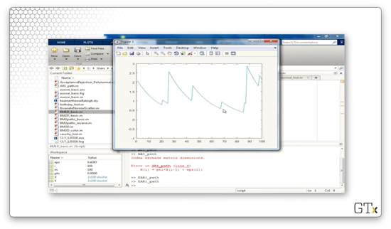
Now let's increase phi to 0.95 and look at the plot again. As we saw previously, we see what looks like exponential decay punctuated by random jumps.
Queueing (OPTIONAL)
In this lesson, we will discuss an easy way to generate random variables associated with queueing processes.
M/M/1
Let's consider a single-server queue with customers arriving according to a Poisson() process. As we know, the interarrival times are iid Exp(), and the service times are iid Exp(). Customers potentially wait in a FIFO queue upon arrival, depending on the state of the server. In general, we require that ; if customers don't get served faster than they arrive, the queue grows unbounded.
In terms of notation, we let denote the interrival between the th and st customer. We let be the th customer's service time, and we let denote the th customer's wait before service.
Lindley Equations
Lindley gives a simple equation for generating a series of waiting times where we don't need to worry about the exponential assumptions. Here's how we generate the st queue time:
This expression makes sense. If the th customer waited a long time, we expect the st customer to wait a long time. Similarly, if the th customer has a long service time, we expect the st customer to wait a long time. However, if the st interarrival time is long, perhaps the system had time to clear out, and the customer might not have to wait so long. Of course, wait times cannot be negative.
We can express the total time in the system for customer as . Here's how we generate :
Customer has to wait until customer clears out of the system, which occurs in time. Then, customer must remain in the system for their service time, .
Brownian Motion
In this lesson, we'll look at generating Brownian motion, as well as a few applications. Brownian motion is probably the most important stochastic process out there.
Brownian Motion
Robert Brown discovered Brownian motion when he looked at pollen under a microscope and noticed the grains moving around randomly. Brownian motion was analyzed rigorously by Einstein, who did a physics formulation of the process and subsequently won a Nobel prize for his work. Norbert Wiener establishes mathematical rigor for Brownian motion: Brownian motion is sometimes called a Wiener process.
Brownian motion is used everywhere, from financial analysis to queueing theory to chaos theory to statistics to many other operations research and industrial engineering domains.
The stochastic process, , is standard Brownian motion if:
- has stationary and independent increments.
Let's talk about the first two points. A standard Brownian motion process always initializes at zero, and the distribution of the process, evaluated at any point, , is Nor(0, ). This result means that a Brownian motion process has a correlation structure.
An increment describes how much the process changes between two points. For example, describes the increment from time to time . If a process has stationary increments, then the distribution of how much the process changes over an interval from to only depends on the length of the interval, .
We can recall our discussion of stationary increments from when we talked about arrivals. For example, if the number of customers arriving at a restaurant between 2 a.m and 5 a.m has the same distribution as the number of customers arriving between 12 p.m and 3 p.m, we would say that the customer arrival process has stationary increments.
Now let's talk about independent increments. A process has independent increments if, for , is independent of .
How do we get Brownian motion? Let's let be any sequence of iid random variables with mean zero and variance one. Donsker's Central Limit Theorem says that:
Remember that denotes convergence in distribution as gets big and denotes the floor or "round down" function: .
When we learned the standard central limit theorem, was equal to one, and the 's converged to a Nor(0,1) random variable. Note that . As we can see, Donsker's central limit theorem is a generalization of the standard central limit theorem, as it works for all . Not only that, but this central limit theorem also mimics the correlation structure of all the 's. Instead of converging to a single random variable, this sum converges to an entire stochastic process for arbitrary .
Let's look at an easy way to construct Brownian motion. To construct 's that have mean zero and variance one, we can take a random walk. Let's take , each with probability . Let's take of at least 100 observations. Then, let and calculate , according to the summation above. Another choice is to simply sample .
Let's construct some Brownian motion. First, we pick some "large" value of and start with . Then:
Miscellaneous Properties of Brownian Motion
As it turns out, Brownian motion is continuous everywhere but is differentiable nowhere.
The covariance between two points in a Brownian motion is the minimum of the two times: . We can use this result to prove that the area under from zero to one is normal:
A Brownian bridge, , is conditioned Brownian motion such that . Brownian bridges are useful in financial analysis. The covariance structure for a Brownian bridge is . Finally, the area under from zero to one is normal:
Geometric Brownian Motion
Now let's talk about geometric Brownian motion, which is particularly useful in financial analysis. We can model a stock price, for example, with the following process:
Let's unpack some of these terms. Of course, is the Brownian motion, which provides the randomness in the stock price. The term refers to the stock's volatility, and is related to the "drift" of the stock's price. Long story short: don't buy a stock unless it is drifting upward. The quantity relates the stock's drift to its volatility, and we want this quantity to be positive. Finally, is the initial price.
Additionally, we can use a geometric Brownian motion to estimate option prices. The simplest type of option is a European call option, which permits the owner to purchase the stock at a pre-agreed strike price, , at pre-determined expiry date, . The owner pays an up-front fee for the privilege to exercise this option.
Let's look at an example. Say that we believe that IBM will sell for $120 per share in a few months. Currently, it's selling for $100 per share. It would be nice to buy 1000 shares of IBM at $100 per share today, but perhaps we don't have $100,000 on hand to make that purchase. Instead, we can buy an option today, for maybe $1.50, that allows us to buy IBM at $105 per share in a few months. If IBM does go to $120 per share, we can exercise our option, instantaneously buying IBM for $105 and selling for $120, netting a $13.50 profit ($15 minus the option price, $1.50).
If the stock drops to, say, $95 per share, then we would choose simply not to exercise the option. Obviously, it doesn't make sense to buy IBM for $105 per share using the option when we can just go to the market and buy it for less.
The question then becomes: what is a fair price to pay for an option? The value, of an option is:
The expression is the profit we make from exercising an option at time , which we bought for dollars. Since we never consider taking a loss, we only consider the difference when it is positive: .
Instead of buying the option, we could have put the money we spent, $1.50, into a bank, where it would make interest. In purchasing the option, we have to pay a penalty of , where is the "risk-free" interest rate that the government is currently guaranteeing.
We can calculate to determine what the option is worth. For example, if we determine that the option is worth $1.50, and we can buy it for $1.30, then perhaps we stand to make some profit.
Alternatively, we can use the option merely for an insurance policy. Southwest airlines bought options on fuel prices many years ago. The fuel prices went way up, and Southwest made a fortune because they could buy fuel at a much lower price.
To estimate the expected value of the option, we can run multiple simulation replications of and and then take the sample average of all the 's. All we need to do is select our favorite values of , , , and , and we are off to the races.
Alternatively, we can just simulate the distribution of directly. Since , we can use a lognormal distribution to simulate directly. Furthermore, we can look up the answer directly using the Black-Sholes equation.
How to Win a Nobel Prize
Let and denote the Nor(0,1) pdf and cdf respectively. Moreover, let's define a constant, :
The Black-Sholes European call option value is:
DEMO
In this demo, we will generate some Brownian motion. Here's ten steps of Brownian motion in one dimension.
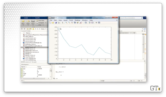
Here's another sample path.
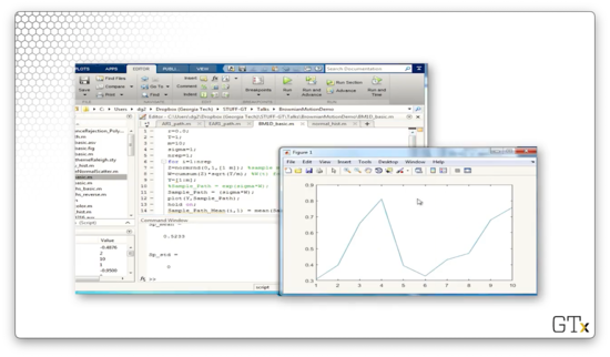
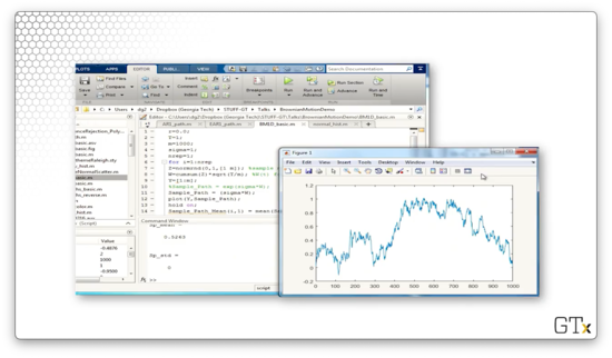
Let's take 1000 steps.
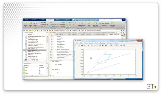
Let's generate ten steps of two-dimensional Brownian motion.
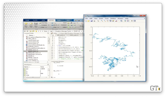
Here's 1000 steps.
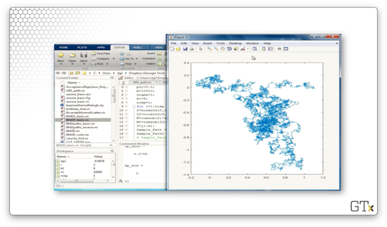
Here's 10000 steps.
Finally, let's look at Brownian motion in three dimensions.
OMSCS Notes is made with in NYC by Matt Schlenker.
Copyright © 2019-2023. All rights reserved.
privacy policy