Simulation
Hand and Spreadsheet Simulations
49 minute read
Notice a tyop typo? Please submit an issue or open a PR.
Hand and Spreadsheet Simulations
Stepping Through a Differential Equation
In this lesson, we are going to solve a differential equation by hand.
Stepping Through a Differential Equation Numerically
If is continuous, then the derivative at - assuming that it exists and is well-defined for any - is:
Note that we also refer to the derivative at as the instantaneous slope at . The expression represents the "rise", and represents the "run". As , the slope between and approaches the instantaneous slope at .
Thus, for small :
We can manipulate this expression to get the following approximation:
Example
Let's suppose that we have a differential equation - perhaps of some population growth model - of the form: , with an initial condition that . We are going to find an approximate solution to this differential equation using a fixed-increment time approach with . This approach is known as Euler's method.
Let's approximate , using the relationship between and from the differential equation:
We can repeat this exercise for . First:
What do we know about ? Let's plug back in to our approximation for , using as and as . Consider:
Recall the approximation for that we just found, and remember that . So:
Again, we have an term that we can substitute for:
If we go through this approximation again and again, we will see the following formula arise:
This strategy works well, although it may deteriorate as gets large since we are compounding approximations (and thus propagating approximation errors) as a function of .
Now, If we plug in , to the generalized equation above, we have:
Now, the precise solution for this differential equation is . We can use a Taylor series to express :
Let's take the first two terms:
Note that for small values of both and .
Let's see how well the approximation performs as we increase . Remember that, for any , . Therefore:
As we can see, our approximation works quite well.
Monte Carlo Integration
In this lesson, we are going to look at how we can use random numbers to perform integration. This technique is known as Monte Carlo integration and is used in many disciplines - from physics to finance - to find integrals that cannot be computed analytically.
Integration
A function, , having derivative is called the antiderivative. The antiderivative, also referred to as the indefinite integral of , is denoted .
The fundamental theorem of calculus states that if is continuous, then the area under the curve for is given by the definite integral:
Monte Carlo Integration
Let's integrate an arbitrary (continuous and well-defined) function, from to :
However, we'd like to integrate from to instead of from to for reasons that will make sense shortly. We can accomplish this limit change using the following substitution:
Thus, and . Additionally, and this is what gets us our limit change, when , , and, when , . Putting the whole thing together, we get:
Of course, we can often compute these types of integrals using the analytical methods we learned in calculus. Alternatively, we can use numerical methods like the rectangle and trapezoid rules or something more exotic like Gauss-Laguerre integration. However, if these methods aren't possible, we can always use Monte Carlo integration.
Suppose that we have a random sample, . Let's define a random variable, , as:
Note that this expression looks precisely like the interior of the integral above, except that is evaluated at , not .
Given our random sample, let's find the sample mean, :
What we'd like to do now is demonstrate that is an effective estimator for . We can appeal to the Law of Large Numbers, which says that if an estimator is asymptotically unbiased and its variance goes to zero, then it's a good estimator.
Let's see if is unbiased for . First, we take the expected value:
Note that, since the 's are iid, the summation and the cancel out:
Remember the Law of The Unconscious Statistician:
Therefore:
Notice that is the pdf of the distribution. This pdf is only defined over and is equal to . So:
We can see that, since , then is an unbiased estimator for . Additionally, it can be shown that , where means that as . With these two conditions met, the Law of Large Numbers implies that as . In short, is an effective estimator for , given a large enough .
Approximate Confidence Interval for
We can also approximate a confidence interval for . Using the central limit theorem, we can see that:
This result suggests that a reasonable confidence interval for is:
Remember from the statistics boot camp that is the standard normal quantile, parameterized by . Also remember that is the sample variance of the 's, defined as:
Example
Suppose . Let's start our approximation by taking the random sample :
Let's define and reduce, taking note that and :
Now let's compute the sample mean, , which we have previously demonstrated is a good estimator for :
Of course, we know that the precise value for is , but our estimation is not far off. Though to be fair, we cheated in our selection from the : notice how nice and spread out the values are.
Now let's compute the approximate confidence interval for . First, let's calculate the sample variance, :
Now, given , we can compute the confidence interval:
This confidence interval is "fat", given that we created it from just four samples. Confidence intervals usually improve as increases, though sometimes convergence is choppy due to good or bad luck with respect to randomness.
Demo
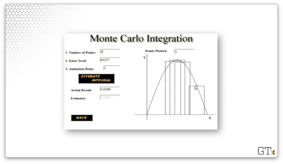
Let's look at a demo for estimating . We've seen this application in a previous lesson. Basically, we are going to draw random rectangles, each with width and centered about a point, , with height . We will add up the areas of the rectangles to approximate the integral.
Here is an approximation, , using rectangles.
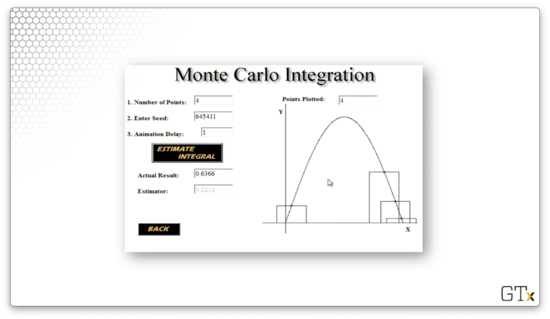
Here is another approximation, , using rectangles. What a terrible estimate!
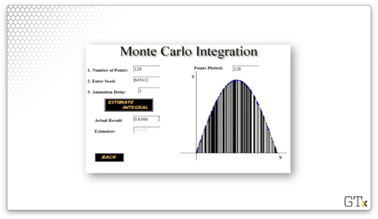
Remember that we can improve our approximation by taking more samples. Here is a third approximation, , using rectangles. Much better.
Let's see how we would run this simulation in Excel. Consider the following spreadsheet.
In the first column, we draw our iid random variables with the RAND() function. In the second column, we generate our 's: . In the third column, we compute , the sample mean. For this example, when , .
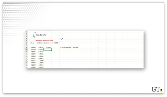
Let's try a slightly more complicated example that we can't integrate easily:
Consider the following spreadsheet, focusing only on the "Random Riemann Sum" section.
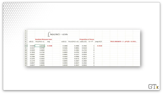
Again, we go through the same process. In the first column, we draw our iid random variables with the RAND() function. In the second column, we generate our 's: . In the third column, we compute , the sample mean. For this example, when , . The true value of the integral is , so our approximation was close.
Making Some Pi
In this lesson, we are going to use Monte Carlo simulation to estimate . This approach is slightly different than Monte Carlo integration, but it uses the same general techniques.
Description
Consider a unit square (with area one, by definition). Inside the square, we inscribe a circle with radius (with corresponding area ). Suppose that we toss darts randomly at the square. The probability that a particular dart lands in the inscribed circle is obviously . We can use this fact to estimate .
Let's toss darts at the square and calculate the proportion, , of darts that land in the circle. From this proportion, we can estimate using . Using the law of large numbers, we know that as .
For instance, suppose that we throw darts at the square and land in the circle. Then , and our estimate for for is . Not bad.
Simulation
Consider the following simulation.
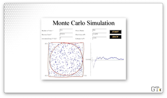
Like we discussed, we throw darts at the square - , in this case - on the left and then use four times the proportion of darts that hit the circle as an estimator for . Our estimate was in this simulation. Note the running estimate for on the chart on the left. As we include more observations, the estimate begins to converge.
Let's see what happens when we increase to .
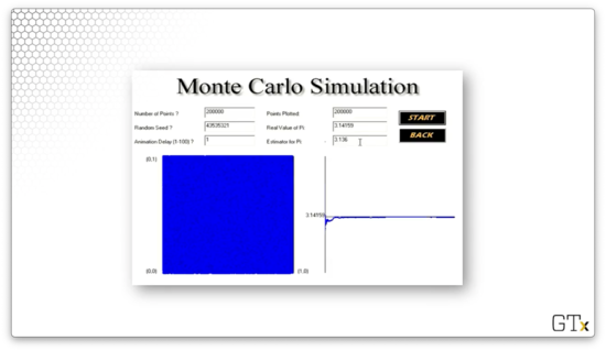
In this example, we've completely covered the square with darts. Our estimate for is , and we can see what appears to be convergence in the chart on the right.
Conducting the Experiment
How do we actually conduct this type of experiment?
To simulate a dart toss, suppose we draw two random variables, . The ordered pair represents the random position of the dart on the unit square. The dart lands in the inscribed circle if:
We can generate such pairs of uniforms and compute the proportion of those that satisfies this inequality. From there, we multiply by four, and we have . For example, suppose we generate uniforms, and are inside the circle. Then .
A Single Server Queue
In this lesson, we will simulate the line that forms in front of the single server at the bakery. This example is going to be our first simulation model that involves non-static customers arriving and receiving service.
Description
Suppose that customers arrive at a single-server queue with iid interarrival times and receive service according to iid service times. Customers must wait in a FIFO (first-in-first-out) line if the server is busy. As the server processes customers, the line advances one customer at a time.
We will simulate this single-server queue setup and then estimate particular performance characteristics of the system, such as:
- the expected customer waiting time
- the expected number of people in the system
- the expected server utilization (proportion of time server spends serving)
Of course, these metrics all matter in the real world. For example, a customer may decide against shopping at a store that has a high expected waiting time. A store owner might not be able to fit a large number of people in their store, and therefore may need the expected number of people in the system to be low. Additionally, a store owner might look at server utilization when considering adding or removing a server.
Notation
The interarrival time between customers and is . Customer 's arrival, , is the sum of all of the preceding interarrival times:
Customer starts service at time . In other words, customer is going to start service at either his arrival time, , or when the customer ahead of him leaves, , whichever is later. We can think of as the departure time of customer .
Customer 's waiting time, , is equal to the service time minus the arrival time: . Similarly, customer 's time in the system, , is equal to the departure time minus the arrival time: .
Customer 's service time is , which we will generate randomly along with interarrival times. Finally, customer 's departure time equals the time that service starts plus the service time: .
Example
Consider the following table of events:
Let's walk through a few customer journeys. Customer one has an interarrival time, , and, assuming that we start the simulation at time , he arrives at time . Since there is no one in from of him, he starts service at , which means his wait time is . His randomly generated service time is , which means his departure time is .
Meanwhile, we have randomly selected an interarrival time, , for customer two. Since customer one arrived at , customer two arrives one minute later at . Now, when does customer two start service? He has to wait for customer one to leave, which happens at . Six minutes have elapsed since customer two arrived, so . We randomly generate a service time , so customer two departs at .
We randomly selected an interarrival time, , for customer three, who arrives at . Customer three has to wait to be served until , at which point he has waited minutes. His service time is drawn randomly at minutes, and he departs at .
Average Waiting Time
We can compute the average waiting time for these six customers by taking the average of the 's:
Average Number of Customers in the System
Now we'd like to compute the average number of customers in the system, which includes both folks in line and in service. Note that the only possible times that the number of customers in the system, , can change is an arrival or a departure time.
These times (and the associated things that happen) are called events, and the type of simulation that we are looking at is discrete event simulation.
Let's look at the following table of events. The first column shows the time that the event occurred. The second column shows the name of the event(s) that occur at that time. The third column shows the number of people in the system, , after the event(s) occurs.
Note that, as a technicality, the first event is the start of the simulation, which occurs at time . There are no people in the system when the simulation starts, so .
The first time anything interesting happens is at time , when customer one arrives. Since this customer is the first in the system, . Nothing changes until time , when customer two arrives. At this point, one customer is being served, and one customer is in line, so . At time , customer three arrives. Since neither customer two nor customer one has left the system, customer three gets in line, and .
Notice that at time , two events occur simultaneously: customer one departs and customer four arrives. Usually, we handle departures before arrivals because we like to clean people out of the system; regardless, the net effect is that is unchanged from . Of course, in real life, customers rarely depart and arrive simultaneously because arrival times and departure times are not usually marked in integer minute increments.
Eventually, the system clears out at time , when customer six departs. As a result, .
Average Number of Customers in the System (Graph)
Consider the following graphical representation of the queue. The x-axis measures time , and the y-axis corresponds to . Each rectangle represents a customer, and the number of customers stacked at any given time-step, , is . The integer subscripts below the x-axis mark events, and the bottom row of rectangles represents the customer receiving service during that interval.
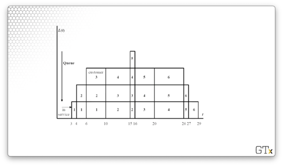
At time , customer one shows up and immediately begins to receive service. At time , customer two arrives and joins the end of the queue while customer one is in service. At time , customer three shows up and the queue has a depth of three. At time , we can see that customer one leaves and customer four arrives, and is unchanged from as customer two begins service.
We can formulate an equation for the average number of people in the system, :
How do we take the integral of such a "weird-looking" function, like ? As it turns out, is a step function, and we integrate a step function by adding up the integrals of all the steps. In this case, we just add up the areas of the rectangles. We can add them up individually or take vertical or horizontal slabs.
Let's take horizontal slabs as an example. The bottom rectangle has height and width . The rectangle above it has height and width . The rectangle above that has height and width . Finally the rectangle on top has height and width . Taken together, the area under between and equals .
Average Number of Customers in the System (Alternate)
Another way to compute the average number of customers in the system is to compute the total customer time in the system and divide that by the total time. We defined a customer's time in the system, , as the difference between their arrival time and departure time: . Therefore:
Server Utilization
Finally, we can obtain the estimated server utilization by looking again at the graph of . The simulation runs for minutes, and the server is giving service for minutes, so the estimated server utilization is .
LIFO
Let's do another example, using the same arrival and service times, but with a last-in-first-out (LIFO) structure instead of first-in-first-out (FIFO).
Compare this table with the previous: all of the 's, 's, and 's are the same. However, in this example, customers at the end of the queue are served before customers at the head.
For example, consider customer two (nothing changes with customer one). Customer two shows up while customer one is receiving service, but customer three shows up before customer two can begin service. Additionally, customer four shows up before customer one leaves. Since this is a LIFO structure, customer four begins to receive service when customer one is complete, at time .
Customer four receives service in six minutes, so he leaves at time . However, customer five has shown up, so his service begins before customer three's service. Customer five receives service in one minute and departs at time , at which point customer three starts service.
Customer three receives service in four minutes, during which customer six has arrived. Customer three departs at time and, two minutes later, customer six departs at time . Finally, customer two receives service in six minutes and leaves at time .
As it turns out, the average waiting time using a LIFO structure is (as compared to ), and the average number of people in the system turns out to be (as compared to ). Thus, in this case, LIFO appears to be a better structure than FIFO, at least concerning these metrics.
An (s, S) Inventory System
In this lesson, we will focus on a more challenging simulation example: an (s, S) inventory system. After this example, we'll have an understanding of why we don't want to run complex simulations by hand.
Description of (s, S)
Let's suppose that a store sells some product at per unit. The inventory policy is to have a least units in stock at the start of each day. If the stock slips to less than by the end of the day, we place an order with our supplier to push our stock up to by the beginning of the next day.
There are various costs associated with this policy. For example, it costs us money to order inventory from our supplier. Additionally, there will be a penalty cost if we fail to satisfy customer demand. As well, there is a holding cost if we stock more inventory than we should.
Notation
Let denote the inventory we have in store at the end of day , and let denote the amount of inventory we order at the end of day . Since we want to top off our inventory to units if falls below , then:
If an order is placed to the supplier at the end of day , it costs the store . We incur cost just for calling up the supplier and nagging them for more product. Additionally, we incur the unit cost times; for example, if we have to order 17 items, this cost is .
Moreover, we incur a cost of /unit to hold unsold inventory overnight. We can think of this cost both in literal terms - refrigerating an item overnight costs a certain amount of electricity - or in terms of opportunity cost - had we not purchased that inventory, we could have put the money elsewhere.
Finally, we incur a penalty cost of /unit if demand can't be met. If we run out of products and a customer cannot make a purchase, perhaps they get mad and damage the store or simply don't return to make purchases.
In this example, we aren't going to allow any backlogs. If a customer comes in and we don't have the products that they want on hand, we cannot satisfy their demand.
The only random component in this example is the demand on day , .
Daily Profit
In English, the total profit for a given day is the sales revenue we generate minus the three costs we incur: ordering cost, holding cost, and penalty cost. Let's translate this expression into a formal equation.
First, what is the total sales revenue? Well, given demand , we can make either sales, or we can sell out our entire inventory, whichever is smaller. For example, if the demand is 15 units, but we only have ten units in inventory, we can only sell ten units. At /unit, we can express this revenue as:
What is the ordering cost? If falls below , it is , where and is the unit cost. Otherwise, the order cost is zero. In other words:
What is the holding cost? It's /unit times the inventory we have at the end of day , :
What is the penalty cost? Well, if the inventory is greater than or equal to the demand, then our penalty cost is nothing: we've completely satisfied customer demand. Otherwise, we incur at penalty cost at /unit for each product greater than our inventory demanded:
As a final piece, what is the inventory at the beginning of day ? It's merely the inventory at the end of the day , , plus the order placed at the end of that day: .
Thus, for a given day , we express the total profit, , as:
Example
Let's look at an example of an inventory system. Suppose we sell each unit at and we purchase each unit at . Further, suppose that we incur a fixed ordering cost , a holding cost per unit, and a penalty cost per unit.
Additionally, consider the following sequence of randomly generated demands:
Finally, let's suppose we start with an initial stock, .
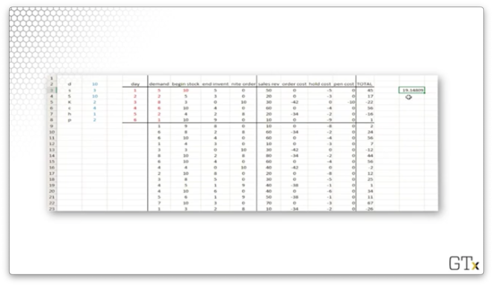
Consider the following table, which tracks inventory, demand, orders, revenue, costs, and profit over six days:
On day one, we start with ten units in stock, and we experience a demand for five units. Therefore, our inventory at the end of the day, , equals . Because , we don't place an order, so . Our sales revenue is , our order cost is , our holding cost is , and our penalty cost is . Finally, our profit for the day is .
At the beginning of day two, we have five items in stock, and we experience a demand for two units. Therefore, our inventory at the end of the day, , equals . Because , we don't place an order, so . Our sales revenue is , our order cost is , our holding cost is , and our penalty cost is . Finally, our profit for the day is .
At the beginning of day three, we have three items in stock and we experience a demand for eight units. Therefore, our inventory at the end of the day, , equals . Because , we place an order for units, so . Our sales revenue is , our order cost is . Our hold cost is , because we have no items in stock, and our penalty cost is because we couldn't satisfy the demand for five units. Finally, our profit for the day is .
Demo
This demo expands on the example we just discussed for an additional days or so. There isn't really any new information to summarize here. Below is a screenshot of the spreadsheet, which you can download from Canvas.
Simulating Random Variables
In this lesson, we will be simulating specific random variables. Much of this material in this lesson was covered in the boot camps.
Discrete Uniform Example
For the simplest example, let's consider a discrete uniform distribution, , from to : . Let with probability for . This example might look complicated, but we can think of it basically as an -sided die toss.
If is a uniform random variable - that is, - we can obtain through the following transformation: , where is the "ceiling", or "round up" function.
For example, suppose and . If , then .
Another Discrete Random Variable Example
Let's look at another discrete random variable. Consider the following pmf, for :
We can't use a die toss to simulate this random variable. Instead, we have to use the inverse transform method.
Consider the following table:
In this first column, we see the three discrete values that can take: . In the second column, we see the values for as defined by the pmf above. In the third column, we see the cdf, , which we obtain by accumulating the pmf.
We need to associate uniforms with -values using both the pmf and the cdf. We accomplish this task in the fourth column.
Consider . and . With this information, we can associate the uniforms on to . In other words, if we draw a uniform, and it falls on - which occurs with probability 0.25 - we select , which has a corresponding of 0.25.
Consider . and . With this information, we can associate the uniforms on to . In other words, if we draw a uniform, and it falls on - which occurs with probability 0.1 - we select , which has a corresponding of 0.25.
Finally, consider . and . With this information, we can associate the uniforms on to . In other words, if we draw a uniform, and it falls on - which occurs with probability 0.65 - we select , which has a corresponding of 0.65
For a concrete example, let's sample . Given a function, that maps -values to the associated set of uniforms, we can compute, , given , by taking the inverse: . For instance, suppose we draw . Since , .
Inverse Transform Method
Let's now use the inverse transform method to generate a continuous random variable. Consider the following theorem: if is a continuous random variable with cdf, , then the random variable .
Notice that is not a cdf because is a random variable, not a particular value. itself is a random variable distributed as .
Given this theorem, we can set , and then solve backwards for using the inverse of : . If we can compute , we can generate a value for given a uniform.
For example, suppose we have a random variable . The cdf of is given by the function . Correspondingly, . However, we also know, according to the theorem, , so . Let's solve for :
What's the point? Computer programs give us one particular type of randomness. When we use RAND() in Excel, or random.random in Python, we always get a random variable . We have shown here that we can take this random variable - the one tool we have available to us - and transform it into any other type of random variable we want. In this particular example, we have shown how to transform into .
Generating Uniforms
All of the examples that we have looked at so far require us to generate "practically" independent and identically distributed (iid) random variables.
How do we do that? For the less programmatically savvy, one way is to use the RAND() function in Excel.
Alternatively, we can use an algorithm to generate pseudo-random numbers (PRNs); in other words, a series of deterministic numbers that appear to be iid . Pick a seed integer, , and calculate:
A given value of exists on . To transform a given into the corresponding , which exists on , we use the following formula:
Here is how we might program this RNG in Python:
# Tested with Python 3.8.3
# I've done this with a generator. There is probably a better way. I am not a Python expert.
def rng(seed):
x_i = seed
while True:
x_i = 16807 * x_i % (2 ** 31 - 1)
yield x_i / (2 ** 31 - 1)
gen = rng(12345678)
print(next(gen)) # 0.621834785967057
print(next(gen)) # 0.17724774832709123
print(next(gen)) # 0.0029061334221186738
print(next(gen)) # 0.84338442554855
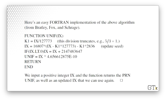
print(next(gen)) # 0.762040194478836Alternatively, we can use this Fortran implementation.
Demo
In this demo, we will generate exponential random variables using the inverse transform method.
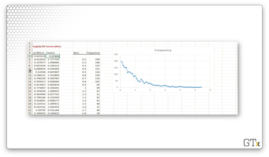
In the first column, we generate several thousand uniform random variables using the RAND() function. In the second column, we apply the inverse transform method to transform these uniforms into exponential random variables using the following equation, which we derived earlier:
Note that since we are looking at exponential random variables for which , the transformation equation simplifies:
On the right-hand side of the spreadsheet, we have constructed a histogram using the exponential random variables with bins of width going from to .
Unsurprisingly, the graph resembles that of the pdf for the exponential distribution with . Additionally, the observed mean value is , which is quite close to the expected value of this distribution: .
Spreadsheet Simulation
In this lesson, we will conduct a spreadsheet simulation. These spreadsheets are very useful in business and other applications, and we can use them in certain discrete-event scenarios, such as an MM1 queue.
Stock Portfolio
We are going to simulate a fake stock portfolio consisting of six stocks from different sectors. We will start out with worth of each stock, and a stock increases or decreases in value each year according to this expression:
The first normal term describes the behavior of stock . For example, if we are looking at a telecommunications stock, we might expect this stock to increase in value, on average, by 8%, so might be . On the other hand, the stock might also be highly volatile, so we might expect the standard deviation of the returns might be 20%: .
The second normal term captures market movement as a whole. Stocks tend to move with the market. Perhaps the entire market is up for all stock sectors, or perhaps it is a bad year, and the whole market is down. In this case, the market on average stays about the same - - but it experiences high volatility: .
Of course, stock prices can't dip below zero. As a result, we have to take the maximum of zero and the computed stock price to ensure that we don't calculate a negative value.
Generating Normals in Excel
To generate a normal random variable in Excel, we can use the following command:
NORM.INV(RAND(), mu, sigma)Remember that RAND() gives us a uniform random variable between and , so we are essentially using the inverse transform method here to turn a uniform random variable into a normal random variable parameterized by mu and sigma.
Example
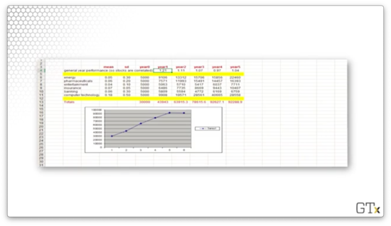
Consider the following spreadsheet.
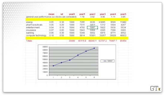
For each sector, we can see the mean and standard deviation for the expected returns in the first two columns. For example, energy has an expected return of but has a standard deviation of .
Across the top, we see the overall market movement. For these five years, the market returned , , , , and .
For each sector, we can see the year over year returns, and we can see the total portfolio returns at the bottom of each year column. Finally, we see the final portfolio value in the bottom-left cell, and we see a chart plotting the portfolio performance below.
Our portfolio performed excellently for this particular simulation: starting with and ending with marks an almost return.
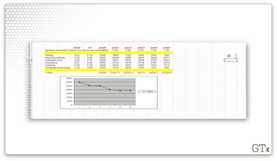
Notice that both the yearly performances of the individual stocks, as well as the yearly market performances, are normal random variables. If we rerun the simulation, these values will change, and we should expect to see a different overall portfolio performance.
Let's look at a second simulation. We did even better this time, returning on a investment.
Let's look at a final example. This time, we lost money. We started with and lost more than a third, ending at .
We can repeat this experiment thousands of times and generate statistics to describe this portfolio.
OMSCS Notes is made with in NYC by Matt Schlenker.
Copyright © 2019-2023. All rights reserved.
privacy policy