Simulation
General Simulation Principles
20 minute read
Notice a tyop typo? Please submit an issue or open a PR.
General Simulation Principles
Steps in a Simulation Study
In this lesson, we will look at the different steps involved in a simulation study.
Problem Formulation
The first step in a simulation study is a high-level problem formulation or problem statement. For example, a problem might be that profits are too low or that customers are complaining about the long lines. Note that the problem statement is often quite general.
Objectives and Planning
In the second step, we focus on objectives and planning. Here we try to consider the specific questions we want to answer to attack the problem we defined. For example, we might want to know how many workers to hire or how much buffer space to insert in the assembly line. By answering these questions, we can potentially mitigate our problem.
Model Building
In step three, we look at model building. We might be interested in an M/M/k queueing model, and so we might be curious about interarrival times, service times, and server counts. Alternatively, we might be modeling natural phenomena that may require us to revisit physics equations.
Sometimes, we combine several models to form a supermodel. The model building process isn't strictly about math; instead, it's both an art and a science that combines rigor, experience, and creativity.
Data Collection
Data collection comes next. Here we think about what kinds of data we need. This consideration will often include specific data points of interest as well as understanding the general characteristics of the data. For example, are we looking at discrete or continuous data?
Additionally, we have to understand how much data we need and whether we can reconcile that need against our budget. Usually, more data is better, and clean data is better than that, but data collection and processing is often a big, expensive task.
Coding
At this point, it's time to start coding. There are many simulation languages to choose from and even more general-purpose programming languages - C++, Python, etc. - that may be sufficient.
Regardless of language choice, we have to consider the modeling paradigm, which describes, at a high level, how we reason about the simulation. Two examples of such paradigms are event-scheduling and process-interaction.
Verification
After we've written at least the first iteration of code, we turn to verification. In this step, we make sure that our program works as expected. In the case of obvious programming errors, we return to the coding step.
Validation
More importantly, we also need to focus on validation. Did we choose the right model? For example, if we modeled a particular system as a simple MM1 queueing system, yet we have five servers instead of one, the answer is "no". Usually, we can show that we have chosen the wrong model using certain statistical techniques. If our model is incorrect, we have to go back to the modeling and data collection steps.
Experimental Design
Once the code has been verified, and the model has been validated, it's time to look at experimental design. In this phase, we think about what experiments we need to run to answer our questions efficiently.
When working on experimental design, we need to think about both statistical considerations - how many experimental runs should I complete to answer my question with high confidence? - as well as time and budget constraints.
Experimental Runs
Once the designs are complete, it's time to run experiments. We press the "go" button and start executing the experiments that we just designed. Often, these experiments take a lot of time to complete.
Output Analysis
After conducting the experiments, we turn to output analysis. We have to perform correct, relevant statistical analysis of the data we gathered from our experiments. This process is often performed iteratively, in conjunction with the experimental design and execution steps. As a general rule, we almost always need more experimental runs.
Implementing Results
Finally, we need to write up our reports and implement results. If all goes well, management will be happy, and we'll be happy, too.
Some Useful Definitions
In this lesson, we will learn some easy definitions that are relevant to all general simulation models. We will use these definitions throughout the rest of the course, and they will be especially important when we look at programming simulations.
System/Entities
A system is a collection of entities - people, machines, things - that interact together to accomplish a goal.
Model
A model is an abstract representation of a system. Usually, the model contains certain mathematical or logical relationships that describe the system in terms of:
- the entities involved in the system
- the various states and state transitions of the system
- the events that can occur in the system
As a basic example, we might model a single-server queueing system using an MM1 queueing model.
System State
The system state is a collection of variables that contains enough information to describe the system at any point in time. We can think of the state as a complete snapshot of the system, containing all the information we need.
Let's look at a single-server queue. At a minimum, we need to keep track of two variables. First, we need to know the number of people in the queue at time , . We also have to keep track of whether the server is busy or idle at time , . If then the server is idle, and if then the server is busy. For a simplistic simulation, knowing these two variables may be sufficient.
Attributes
Entities - customers, resources, servers - can be permanent or temporary. For example, machines in an assembly line are often permanent, whereas individual customers come and go.
Entities can have different properties or attributes. For example, different customers have differing amounts of money to spend, and some customers may have higher priority than others. In queueing systems, individual servers might have various capacities for accomplishing work.
List/Queue
A list (or queue) is an ordered list of associated entities. For example, the line that forms in front of a server is a queue and is often ordered by arrival time.
Event
An event is a point in time at which something interesting happens - that is, the system state changes - that typically can't be predicted with certainty beforehand.
For example, in queueing systems, the time at which a customer arrives is an event. We don't know with certainty when a customer will arrive, but we do know that an arrival changes the state of the system. Similarly, the time at which a customer departs is an event.
Some people regard an event not only as the time that something happens but also the type of thing that happens. Even though an event technically refers to a time, we can also use it to refer to a "what"; for example, an arrival event.
Activity
An activity, also known as an unconditional wait, is a duration of time of specified length. For example, we might say that the times between customer arrivals are exponential or that service times are constant. These events are specified because we have explicitly defined the parameters for generating them.
Conditional Wait
A conditional wait is a duration of time of unspecified length. For example, in a queueing system, we don't know customer wait times directly; in fact, that's often why we are running a simulation. All we can specify when we are programming our simulation are the arrival times and service times. From those specifications, either we or the simulation language has to reverse engineer the waiting times.
Folks will occasionally run simulations and observe the waiting times and forget about the arrival times and service times. As it turns out, it's a lot harder to reverse engineer these variables from the waiting times. As a result, the best strategy is to collect the arrival times and service times.
Time-Advance Mechanisms
In this lesson, we will discuss the simulation clock and how this clock moves the simulation along as time progresses. We can carry out the calculations for the clock ourselves, or the simulation language can do it for us. Regardless, the clock is the heart of any discrete-event simulation.
Definitions
The simulation clock is a variable whose value represents simulated time (not real time). Time-advance mechanisms describe how the simulation clock moves from time to time. The clock always moves forward, never backward, and can advance using two mechanisms: fixed-increment time advance and next-event time advance.
Clock Movement
In the fixed-increment time advance approach, we update the system state at fixed times, where is some small number chosen appropriately. For example, if is minute, then we update the state every minute.
This approach makes sense for continuous-time models, which often contain differential equations and stochastic differential equations, such as models of aircraft movement through space or weather patterns. Additionally, we use this approach in models where data is only available at fixed time units, such as at the end of every month.
This methodology is not emphasized in this course. Suppose we are looking at a queueing model where customers show up every so often and get served every so often. If we are advancing the clock every second, nothing is happening most of the time, and we are just wasting computation cycles.
In the next-event time advance approach, we determine all future events at the beginning of the simulation - time - and we place them in a future events list (FEL), ordered by time. Moving forward, the clock doesn't advance by a fixed increment; instead, it jumps to the most imminent event at the head of the FEL.
For example, at time , we might determine that one arrival occurs at time and the next arrival occurs at . After determining these events, our FEL is a two-element list where the first arrival is the first element and the second arrival is the second.
In this case, the clock advances from time to time and then from to . At each event, both the system state and potentially the FEL are updated.
Note that this approach has the benefit of jumping directly to times where interesting things are happening; in other words, the simulation doesn't have to waste cycles processing time-steps that aren't marked by events.
Notes on FELs
By definition, the system state can only change at event times: nothing happens between events. In queueing systems, in particular, we only care about arrivals and departures, and we don't consider customers standing in line bored to be "anything happening".
As a result, the simulation progresses sequentially by executing - "dealing with" - the most imminent event on the FEL. After dealing with the most imminent event, we advance to the next-most imminent event, and we progress until we reach the end of the FEL.
Imminent Events
As we said, the clock advances to the most imminent event at the head of the FEL. How do we "deal with" this event as programmers? We have to do two things: update the system state and, potentially, update the FEL.
The specific state update depends on the type of event we are processing. For example, if we are looking at an arrival event, and the server is not busy, we have to turn on the server. Alternatively, if the server is busy, the new arrival has to wait, so we enqueue it. A departure event might involve turning a busy server off.
In any case, we might have to update the FEL. For example, when we process an arrival, the first thing we often do is generate the next arrival, which we place at the end of the FEL. Additionally, if a customer receives service upon arrival, we might have to schedule an event marking the completion of this service.
Updating the FEL
Any time the simulation processes an event, it might have to update the FEL. Here are several different operations the simulation might perform on the FEL:
- appending/inserting new events
- deleting events
- rearranging events
- doing nothing
Suppose a customer arrives in the system: an arrival event occurs. As we said, the first step we usually take in processing an arrival is to spawn the next arrival time and place it in the appropriate position in the FEL.
If the new arrival time is sufficiently far in the future, we can append it to the end of the FEL. However, suppose we generated an arrival ten minutes into the future, but a slow server doesn't finish serving the current customer until thirty minutes into the future. In this case, the arrival event precedes the service completion event, and we have to insert the arrival in the interior of the FEL instead of appending it.
Now, suppose we have an arrival of a particularly rowdy customer in the queue. In response to this customer, other customers in line might switch lines or leave the system altogether. For folks who switch lines, their associated events may need to be rearranged within the FEL. If a customer leaves the system completely, any future events linked to them should be deleted from the FEL.
More FEL Remarks
Since we are applying many different operations to the FEL throughout the life of the simulation, we have to make sure that we represent the FEL efficiently. Typically, we use a linked list since it supports more efficient insertion and deletion than typical arrays.
Read more about the time complexity of linked list operations here.
Occasionally we encounter events that occur simultaneously. For instance, suppose a customer shows up at the exact same time that another customer finishes service. Do we deal with the arrival or the departure first?
While there is no right answer, its important to establish ground rules for dealing with ties, so there is no confusion in the middle of the simulation. One strategy is to handle the service completion event before the arrival, getting one customer out of the system before letting another enter.
Almost every commercial discrete-event simulation language maintains an FEL somewhere deep down in its core. If we are writing a simulation in a general-purpose programming language - C++, Python, etc. - we have to maintain the FEL ourselves. If we are using a simulation package, we just have to specify the events, and the language will manage the FEL for us, which saves us a lot of programming time.
Example
Note: this example can be found in Law's book.
Let's look at a simple example of the next-event time advance mechanism. We will consider a single server system containing a FIFO queue that will process exactly ten customers. The arrival and service times for these customers are:
Now, let's see how the simulation unfolds.
In the first column, we see the simulation clock, which we represent with the variable . In the second column, we see the system state, which contains two pieces of data: the number of people in the queue, , and whether or not the server is busy, .
In the third column, we see the queue, a dynamic list ordered by customer arrival times. Each element in the queue is a tuple, where the first element references the customer number, and the second element references their arrival time.
The fourth column holds the FEL. The FEL also contains two pieces of information per entry: the event time and the event type.
Finally, we keep track of some cumulative statistics in the final column. Specifically, we keep track of the total busy time of the server and the total customer time in the system.
At time , we start the simulation. Since no one is in the queue, and the server is idle, . Additionally, the queue is empty. We know that customer one arrives at time , so the FEL has one element, , indicating that customer one (A)rrives at time . Since no one is in the system, our two cumulative statistics are both zero.
Since the most imminent event in our FEL occurs at time , we advance the clock to that time. Since the queue is empty, the customer that arrives immediately receives service, so the queue remains empty, , and the server turns itself on: .
Let's look at the FEL. This arrival event spawns two new events. First, we generate the arrival of customer two at time : . Additionally, we know that customer one receives service in five minutes, from the table above, so we can create their (D)eparture event: .
Additionally, at this time, customer one has just entered the system, so the total busy time and total customer time in the system are still zero.
Since the most imminent event in our FEL now occurs at time , we advance the clock to that time. Since customer one is still receiving service, customer two has to wait in the queue. Thus, , , and the queue is .
Let's look at the FEL. Customer two's arrival spawns one new event, customer three's arrival. We know that customer three arrives at time , so the FEL looks like this: . Note that we cannot generate the departure event for customer two just yet because they haven't started service.
At this point, customer one has been in the system for two minutes, and the server has been serving him for two minutes. As a result, both the cumulative busy time and the total customer time in the system are two.
Two Modeling Approaches
In this lesson, we will look at two high-level simulation modeling approaches, the event-scheduling approach and the process-interaction approach. Of the two, we will use the process-interaction method to model complicated simulation processes for the remainder of the course.
Event Scheduling
In event scheduling, our focus is on the events and how they affect the system state. As the simulation evolves, we have to keep track of every event in increasing order of time of occurrence. This constant bookkeeping and corresponding FEL maintenance is a programming hassle. That said, we might use this approach if we were looking at programming a simulation from scratch in a language like C++ or Python because of its conceptual simplicity.
Generic Event Scheduling Flow Chart
Note: this chart can be found in Law's book.
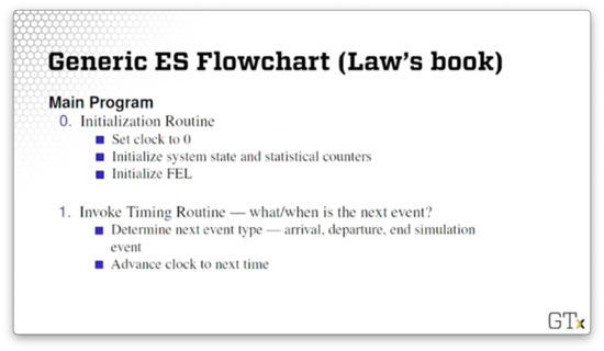
First, we need a main program that supervises everything else. Most importantly, this program invokes three routines: the initialization routine, the timing routine, and the event routine.
We invoke the initialization routine first. Here, we set the clock to zero and initialize the system state, statistical counters, and the FEL. Usually, the FEL initially contains the first arrival event and the event marking the end of the simulation.
Then, we invoke the timing routine. This routine determines when the next event is, what type of event it is - arrival, departure, end of simulation - and then advances the clock to the next event.
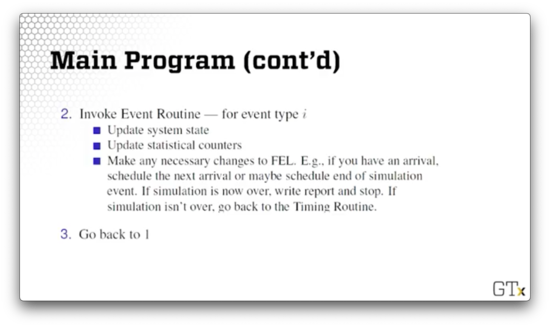
Third, we invoke the event routine itself. First, we update the system state along with our statistical counters, and then we update the FEL appropriately given the event. For example, if the routine is processing an arrival, we might generate another arrival and append or insert it into the FEL. If we are processing the event marking the end of the simulation, we generate any output and end the program; otherwise, we return to the timing routine.
Arrival Event
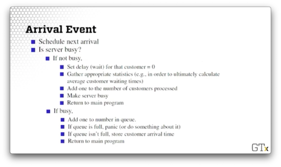
Let's talk about processing arrivals. As we alluded to previously, the first thing we do is schedule the next arrival. Next, we examine the server and see if they are busy.
If the server is not busy, we set the waiting time for the arrived customer to zero, and we update the appropriate statistics - for example, the average customer waiting time. We increment the number of customers who have gone through the line, and we make the server busy. Finally, we return to the main program.
If the server is busy, we add the customer to the queue and increment the number of customers enqueued. If the queue is full, we might have to adjust some parts of the system to accommodate this capacity. Perhaps we kick the customer out. If the queue isn't full, we store the customer arrival time - we will need this later to compute their waiting time. Finally, we return to the main program.
Departure Event
Now let's look at departure events.
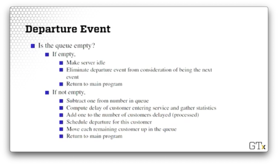
We first check to see if the queue is empty. If it is, we make the server idle since there are no more customers to serve. Additionally, we eliminate the departure event from consideration of being the next event because departures are impossible if there are no customers. Finally, we return to the main program.
If the queue isn't empty, we grab the first guy from the front of the queue and subtract one from the number enqueued. We compute the delay of the customer entering service and gather the appropriate statistics. We schedule his departure, and we shift each remaining customer forward one space in the queue. Finally, we return to the main program.
Process Interaction
As we've seen, the event scheduling approach requires a lot of manual bookkeeping. Now we will look at the process interaction paradigm, which is one of the greatest achievements of modern simulation because it lets us model and program much more seamlessly. We will use this method in class.
In the process-interaction approach, we concentrate on a generic customer or entity and the sequences of events and activities it undergoes as it progresses through the system. The simulation language keeps track of how one generic entity interacts with all the other generic entities. At any time during the simulation, there may be many customers competing with each other for resources.
We have the task of modeling the generic customer, but we don't have to deal with the event bookkeeping, which the simulation package handles deep inside its core. The dirty little secret is that the simulation language is doing event scheduling in its implementation but exposes an API that allows us to model using process interaction.
In queueing simulations, a customer is generated, eventually gets served, and then leaves. How do we perform these actions in a language like Arena? Arena exposes functionality for creating, processing and disposing of entities.
With Arena, we generate customers every once in a while. We process/serve the customers after they wait in line for zero or more time units. Finally, we dispose of the customers after we finish processing them.
Simulation Languages
In this lesson, we will discuss simulation languages themselves in a very generic way.
Simulation Languages
There are more than 100 commercial simulation languages out in the ether. The lower-level languages - FORTRAN, SIMSCRIPT, and GPSS/H - require more programmer work. In contrast, the higher-level languages like Extend, Arena, Simio, Automod, and AnyLogic require a lot less programming effort to get up and running.
There are 5-10 major simulation players in university settings. In industry, the price for simulation packages can range from under $1,000 to more than $100,000. Thankfully, freeware is also available: simulation packages exist in Java and Python (SimPyl). Though they might contain a learning curve, these packages can be powerful and enjoyable to work with.
Selecting a Simulation Language
What factors should we take into account when selecting a language?
We can examine the various costs. For example, we can look at the cost of purchasing the licenses, the cost of specialized programmers, as well as certain run-time costs.
Additionally, we can look at the ease of learning. Different packages may have different learning curves, and each may vary with respect to documentation, syntax, and flexibility.
Furthermore, we can compare packages based on their worldviews. We already discussed why we like process interaction better than event scheduling. If we are looking at continuous systems, we will need a language with continuous modeling capabilities. Often, we need a language that supports a combination of different approaches.
Finally, we have to think about which features we need. Different packages have different random variate generators, statistics collection capabilities, debugging aids, graphics packages, and user communities.
Where can you learn about simulation languages?
- A simulation class (like this!)
- Textbooks, especially in conjunction with a course
- Conferences such as Winter Simulation Conference
- Courses offered by vendors (although these often come at a steep price)
OMSCS Notes is made with in NYC by Matt Schlenker.
Copyright © 2019-2023. All rights reserved.
privacy policy