Happy studying! Did you find my notes useful this semester?
Please consider
giving me a few bucks
or
buying me a beer. Contributions like yours help me keep these notes forever free.
Happy studying! Did you find my notes useful this semester?
Please consider
giving me a few bucks
or
buying me a beer. Contributions like yours help me keep these notes forever free.
Notice a tyop typo? Please submit an
issue
or open a
PR.
Calculus, Probability, and Statistics Primers
Calculus Primer (OPTIONAL)
In this lesson, we are going to take a quick review of calculus. If you are already familiar with basic calculus, there is nothing new here; regardless, it may be helpful to revisit these concepts.
Calculus Primer
Suppose that we have a function, f(x), that maps values of x from a domain, X, to a range, Y. We can represent this in shorthand as: f(x):X→Y.
For example, if f(x)=x2, then f(x) maps values from the set of real numbers, R, to the nonnegative portion of that set, R+.
We say that f(x) is continuous if, f(x) exists for all x∈X and, for any x0,x∈X, limx→x0f(x)=f(x0). Here, "lim" refers to limit.
For example, the function f(x)=3x2 is continuous for all x. However, consider the function f(x)=⌊x⌋, which rounds down x to the nearest integer. This function is not continuous and has a jump discontinuity for any integer x. Here is a graph.
If f(x) is continuous, then the derivative at x - assuming that it exists and is well-defined for any x - is:
dxdf(x)≡f′(x)≡h→0limhf(x+h)−f(x)
Note that we also refer to the derivative at x as the instantaneous slope at x. The expression f(x+h)−f(x) represents the "rise", and h represents the "run". As h→0, the slope between (x,f(x)) and (x+h,f(x+h)) approaches the instantaneous slope at (x,f(x)).
Some Old Friends
Let's revisit the derivative of some common expressions.
The derivative of a constant, a, is 0.
The derivative of a polynomial term, xk, is kxk−1.
The derivative of ex is ex.
The derivative of sin(x) is cos(x).
The derivative of cos(x) is −sin(x).
The derivative of the natural log of x, ln(x) is x1.
Finally, the derivative of arctan(x) is equal to 1+x21
Now let's look at some well-known properties of derivatives. The derivative of a function times a constant value is equal to the derivative of the function times the constant:
[af(x)]′=af′(x)
The derivative of the sum of two functions is equal to the sum of the derivatives of the functions:
[f(x)+g(x)]′=f′(x)+g′(x)
The derivative of the product of two functions follows this rule:
[f(x)g(x)]′=f′(x)g(x)+g′(x)f(x)
The derivative of the quotient of two functions follows this rule:
[g(x)f(x)]′=g2(x)g(x)f′(x)−f(x)g′(x)
We can remember this quotient rule with the following pneumonic, referring to the numerator as "hi" and the denominator as "lo": "lo dee hi minus hi dee lo over lo lo".
Finally, the derivative of the composition of two functions follows this rule:
[f(g(x))]′=f′(g(x))g′(x)
Example
Let's look at an example. Suppose that f(x)=x2 and g(x)=ln(x). From our initial derivative rules, we know that f′(x)=2x and g′(x)=x1.
Let's calculate the derivative of the product of f(x) and g(x):
[f(x)g(x)]′=f′(x)g(x)+g′(x)f(x)
[f(x)g(x)]′=2xlnx+xx2=2xlnx+x
Let's calculate the derivative of the quotient of f(x) and g(x):
[g(x)f(x)]′=g2(x)g(x)f′(x)−f(x)g′(x)
[g(x)f(x)]′=ln2x2xlnx−x
Let's calculate the derivative of the composition f(g(x)):
[f(g(x))]′=f′(g(x))g′(x)
[f(g(x))]′=x2ln(x)
The expression f′(g(x)) might look tricky at first. Remember that f(x)=x2, so f′(x)=2x. Thus, f′(g(x))=2g(x)=2ln(x).
Second Derivatives
The second derivative of f(x) equals the derivative of the first derivative of f(x): f′′(x)=dxdf′(x). We spoke of the first derivative as the instantaneous slope of f(x) at x. We can think of the second derivative as the slope of the slope.
A classic example comes from physics. If f(x) describes the position of an object, then f′(x) describes the object's velocity and f′′(x) describes the object's acceleration.
So why do we care about second derivatives?
A minimum or maximum of f(x) can only occur when the slope of f(x) equals 0; in other words, when f′(x)=0. Mentally visualizing the peaks and valleys of graphs of certain functions may help in understanding why this is true.
Consider a point, x0, such that f′(x0)=0. If f′′(x0)<0, then f(x0) is a maximum. If f′′(x0)>0, then f(x0) is a minimum. If f′′(x0)=0, then f(x0) is an inflection point.
Example
Consider the function f(x)=e2x+e−x. We want to find a point, x0, that minimizes f. Let's first compute the derivative, using the composition rule for each term:
f′(x)=[e2x+e−x]′=2e2x−e−x
Let's find x0 such that f′(x0)=0.
2e2x−e−x=0
2e2x=e−x
e2xe−x=2
ln(e2xe−x)=ln(2)
ln(e−x)−ln(e2x)=ln(2)
−x−2x=ln(2)
−3x=ln(2)
x=−3ln(2)≈−0.231
Now, let's calculate f′′(x):
f′′(x)=[2e2x−e−x]′=4e2x+e−x
Let's plug in x0:
f′′(−0.231)=4e2∗−0.231+e0.231≈3.78
Since this value is positive, f(x0) is a minimum. Furthermore, since ex>0 for all x, f′′(x)>0 for all x. This means that f(x0) is not only a local minimum, but specifically is the global minimum of f(x).
Saved By Zero! Solving Equations (OPTIONAL)
In this lesson, we are going to look at formal ways to find solutions to nonlinear equations. We will use these techniques several times throughout the course, as solving equations is useful in a lot of different methodologies within simulation.
Finding Zeroes
When we talk about solving a nonlinear equation, f, what we mean is finding a value, x, such that f(x)=0.
There are a few methods by which we might find such an x:
Let's remind ourselves of an example from the previous lesson.
Consider the function f(x)=e2x+e−x. We want to find a point, x0, that minimizes f. Let's first compute the derivative, using the composition rule for each term:
f′(x)=[e2x+e−x]′=2e2x−e−x
Let's find x0 such that f′(x0)=0.
2e2x−e−x=0
2e2x=e−x
e2xe−x=2
ln(e2xe−x)=ln(2)
ln(e−x)−ln(e2x)=ln(2)
−x−2x=ln(2)
−3x=ln(2)
x=−3ln(2)≈−0.231
Now, let's calculate f′′(x):
f′′(x)=[2e2x−e−x]′=4e2x+e−x
Let's plug in x0:
f′′(−0.231)=4e2∗−0.231+e0.231≈3.78
Since this value is positive, f(x0) is a minimum. Furthermore, since ex>0 for all x, f′′(x)>0 for all x. This means that f(x0) is not only a local minimum, but specifically is the global minimum of f(x).
Bisection
Suppose we have a function, g(x), and suppose that we can find two values, x1 and x2, such that g(x1)<0 and g(x2)>0. Given these conditions, we know, via the intermediate value theorem, that there must be a solution in between x1 and x2. In other words, there exists x∗∈[x1,x2] such that g(x∗)=0.
To find x∗, we first compute x3=2x1+x2. If g(x3)<0, then we know that x∗ exists on [x3,x2]. Otherwise, if g(x3)>0, then x∗ exists on [x1,x3]. We call this method bisection because we bisect the search interval - we cut it in half - on each round. We continue bisecting until the length of the search interval is as small as desired. See binary search.
Example
Now we are going to use bisection to find the solution to g(x)=x2−2. Of course, we know analytically that g(2)=0, so we are essentially using bisection here to approximate 2.
Let's pick our two starting points, x1=1 and x2=2. Since f(x1)=−1 and f(x2)=2, we know, from the intermediate value theorem, that there must exist an x∗∈[1,2] such that f(x∗)=0.
We consider a point, x3, halfway between x1 and x2: x3=21+2=1.5. Since f(x3)=0.25, we know that x∗ lies on the interval [1,1.5].
Similarly, we can consider a point, x4, halfway between x1 and x3: x4=21+1.5=1.25. Since f(x4)=−0.4375, we know that x∗ lies on the interval [1.25,1.5].
Let's do this twice more. x5=21.25+1.5=1.375. f(x5)=−0.109, so x∗ lies on the interval [1.375,1.5]. x6=21.375+1.5=1.4375. f(x6)=0.0664, so x∗ lies on the interval [1.375,1.4375].
We can see that our search is converging to 2≈1.414.
Newton's Method
Suppose that, for a function g(x), we can find a reasonable first guess, x0, for the solution of g(x). If g(x) has a derivative that isn't too flat near the solution, then we can iteratively refine our estimate of the solution using the following sequence:
xi+1=xi−g′(xi)g(xi)
We continue iterating until the sequence appears to converge.
Example
Let's try out Newton's method for g(x)=x2−2. We can re-express the sequence above as follows:
xi+1=xi−2xixi2−2
xi+1=xi−(2xi−xi1)
xi+1=2xi+xi1
Let's start with a bad guess, x0=1. Then:
x1=2x0+x01=21+11=1.5
x2=2x1+x11=21.5+1.51≈1.4167
x3=2x2+x21=21.4167+1.41671≈1.4142
After just three iterations, we have approximated 2 to four decimal places!
Integration (OPTIONAL)
What goes up, must come down. A few lessons ago, we looked at derivatives. In this lesson, we will focus on integration.
Integration
A function, F(x), having derivative f(x) is called the antiderivative. The antiderivative, also referred to as the indefinite integral of f(x), is denoted F(x)=∫f(x)dx.
The fundamental theorem of calculus states that if f(x) is continuous, then the area under the curve for x∈[a,b] is given by the definite integral:
∫abf(x)dx≡F(x)∣∣∣∣ab≡F(b)−F(a)
Friends of Mine
Let's look at some indefinite integrals:
∫xkdx=k+1xk+1+C,k=−1
∫xdx=ln∣x∣+C
∫exdx=ex+C
∫cos(x)dx=sin(x)+C
∫1+x2dx=arctan(x)+C
Note that C is a constant value. Consider a function f(x). Since the derivative of a constant value is zero, f′(x)=[f(x)+C]′. When we integrate f′(x), we need to re-include this constant expression: ∫f′(x)=f(x)+C.
Let's look at some well-known properties of definite integrals.
The integral of a function from a to a is zero:
∫aaf(x)dx=0
The integral of a function from a to b is the negative of the integral from b to a:
∫abf(x)dx=−∫baf(x)dx
Given a third point, c, the integral of a function from a to b is the sum of the integrals from a to c and c to b:
∫abf(x)dx=∫acf(x)dx+∫cbf(x)dx
Furthermore, the integral of a sum is the sum of the integrals:
∫[f(x)+g(x)]dx=∫f(x)dx+∫g(x)dx
Similar to the product rule for derivatives, we integrate products using integration by parts:
∫f(x)g′(x)dx=f(x)g(x)−∫g(x)f′(x)dx
Similar to the chain rule for derivatives, we integrate composed functions using the substitution rule, substituting u for g(x):
∫f(g(x))g′(x)dx=∫f(u)du, where u=g(x)
Example
Let's look at an example. Given f(x)=x and g′(x)=e2x, let's compute the integral of f(x)g′(x)dx from [0,1].
We know, via integration by parts, that:
∫01f(x)g′(x)dx=f(x)g(x)∣∣∣∣01−∫01g(x)f′(x)dx
Notice that we need to take the integral of g′(x). We can calculate this using u-substitution. Let a(x)=2x and b(x)=ex. Then, using the substitution rule above:
∫b(a(x))a′(x)dx=∫b(u)du, where u=a(x)
Note that a′(x)=2, and b(a(x))=b(2x)=e2x=g′(x). Thus,
∫2g′(x)dx=∫eudu, where u=a(x)
Divide both sides by two:
∫g′(x)dx=21∫eudu, where u=a(x)
Integrate:
g(x)+C=21eu+C, where u=a(x)
Subtract C from both sides and substitute:
g(x)=21e2x
Now that we know g(x), let's return to our integration by parts:
∫01f(x)g′(x)dx=f(x)g(x)∣∣∣∣01−∫01g(x)f′(x)dx
Let's substitute in the appropriate values for f(x), f′(x) and g(x):
∫01xe2xdx=21xe2x∣∣∣∣01−∫0121e2xdx
Let's pull out the 21:
∫01xe2xdx=21(xe2x∣∣∣∣01−∫01e2xdx)
Of course, we already know how to integrate e2x:
∫01xe2xdx=21(xe2x∣∣∣∣01−21e2x∣∣∣∣01)
Now, let's solve:
∫01xe2xdx=21((e2−21e2)−(0−21e0))
∫01xe2xdx=21(2e2+21)
∫01xe2xdx=4e2+41
Taylor and Maclaurin Series
Derivatives of arbitrary order k can be written as f(k)(x) or dxkdkf(x). By convention, f(0)(x)=f(x).
The Taylor series expansion of f(x) about a point a is given by the following infinite sum:
f(x)=k=0∑∞k!f(k)(a)(x−a)k
The Maclaurin series expansion of f(x) is simply the Taylor series about a=0:
f(x)=k=0∑∞k!f(k)(0)∗xk
Maclaurin Friends
Let's look at some familiar Maclaurin series:
sin(x)=k=0∑∞(2k+1)!−1k+1∗x2k+1
cos(x)=k=0∑∞(2k)!−1k∗x2k
ex=k=0∑∞k!xk
While We're At It...
Let's look at some other sums, unrelated to Taylor or Maclaurin series, that are helpful to know.
The sum of all the integers between 1 and n is given by the following equation:
k=1∑∞k=2n(n+1)
Similarly, if we want to add the sum of the squares of all the integers between 1 and n, we can use this equation:
k=1∑∞k2=6n(n+1)(2n+1)
Finally, if we want to sum all of the powers of p, and −1<p<1, we can use this equation:
k=0∑∞pk=1−p1
L'Hôspital's Rule
Occasionally, we run into trouble when we encounter indeterminate ratios of the form 0/0 or ∞/∞. L'Hôspital's Rule states that, when limx→af(x) and limx→ag(x) both go to zero or both go to infinity, then:
x→alimg(x)f(x)=x→alimg′(x)f′(x)
For example, consider the following limit:
x→0limxsin(x)
As x→0, sin(x)→0. Thus, we can apply L'Hôspital's Rule:
x→0limxsin(x)=x→0lim1cos(x)=1
Integration Computer Exercises (OPTIONAL)
In this lesson, we will demonstrate several numerical techniques that we might need to use if we can't find a closed-form solution to a function we are integrating. One of these techniques incorporates simulation!
Riemann Sums
Suppose we have a continuous function, f(x), under which we'd like to approximate the area from a to b. We can fit n adjacent rectangles between a and b, such that each rectangle has a width Δx=(b−a)/n and a height f(xi), where xi = a+iΔx is the right-hand endpoint of the ith rectangle.
The sum of the areas of the rectangles approximates the area under f(x) from a to b, which is equal to the integral of f(x) from a to b:
∫abf(x)dx≈i=1∑n[f(xi)Δx)]
We can simplify the right-hand side of the equation by pulling the Δx term out in front of the sum and substituting in the appropriate values for xi:
Suppose we have a function, f(x)=sin((πx)/2), which we would like to integrate from 0 to 1. In other words, we want to compute:
∫01sin(2πx)
We can approximate the area under this curve using the following formula:
∫abf(x)dx≈nb−ai=1∑nf(a+ni(b−a))
Let's plug in a=0 and b=1:
∫01f(x)dx≈n1i=1∑nf(ni)
Finally, let's replace f:
∫01f(x)dx≈n1i=1∑nsin(2nπi)
For n=100, this sum calculates out to approximately 0.6416, which is pretty close to the true answer of 2/π≈0.6366. For n=1000, our estimate improves to approximately 0.6371.
Trapezoid Rule
Here we are going to perform the same type of numerical integration, but we are going to use the trapezoid rule instead of the rectangle rule/Reimann sum. Under this rule:
∫abf(x)dx≈[2f(x0)+i=1∑n−1f(xi)+2f(xn)]Δx
Substituting a and b simplifies the right-hand side of the formula:
For n=100, this sum calculates out to approximately 0.63661, which is very close to the true answer of 2/π≈0.63662. Note that, even when n=1000, the Reimann estimation was not this precise; indeed, integration via the trapezoid rule often converges faster than the Reimann approach.
Monte Carlo Approximation
Suppose that we can generate an independent and identically distributed sequence of numbers, U1,U2,...,Un, sampled randomly from a uniform (0,1) distribution. If so, it can be shown that we can approximate the integral of f(x) from a to b according to the following formula:
∫abf(x)dx≈nb−ai=1∑nf(a+Ui(b−a))
Note that this looks a lot like the Reimann integral summation. The difference is that these rectangles are not adjacent, but rather scattered randomly between a and b. As n→∞, the approximation converges to an equality, and it does so about as quickly as the Reimann approach.
Example
Suppose we have a function, f(x)=sin((πx)/2), which we would like to integrate from 0 to 1. In other words, we want to compute:
∫01sin(2πx)
We can approximate the area under this curve using the following formula:
∫abf(x)dx≈nb−ai=1∑nf(a+Ui(b−a))
Let's plug in a=0 and b=1:
∫01f(x)dx≈n1i=1∑nf(Ui)
Let's replace f:
∫01f(x)dx≈n1i=1∑nsin(2πUi)
Here is some python code for how we might simulate this:
# Tested with Python 3.8.3from random import randomfrom math import pi, sindefsimulate(n): result =0for _ inrange(n): result +=sin(pi * random()/2)return result / ntrials_100 =sum([simulate(100)for _ in range(100)])/100print(trials_100)trials_1000 =sum([simulate(100)for _ in range(1000)])/1000print(trials_1000)
After running this script once on my laptop, trials_100 equals approximately 0.6355, and trials_1000 equals approximately 0.6366.
Probability Basics
In this lesson, we will start our review of probability.
Basics
Hopefully, we already know the very basics, such as sample spaces, events, and the definition of probability. For example, if someone tells us that some event has a probability greater than one or less than zero, we should immediately know that what they are saying is false.
Conditional Probability
The probability of some event, A, given some other event, B, equals the probability of the intersection of A and B, divided by the probability of B. In other words, the conditional probability of A given B is:
P(A∣B)=P(B)P(A∩B)
Note that we assume that P(B)>0 so we can avoid any division-by-zero errors.
A non-mathematical way to think about conditional probability is the probability that A will occur given some updated information B.
For example, think about the probability that your best friend is asleep at any point in time. Now, consider that same probability, given that it's Tuesday at 3 am.
Example
Let's toss a fair die. Let A={1,2,3} and B={3,4,5,6}. What is the probability that the dice roll is in A given that we know it is in B?
We can think about this problem intuitively first. There are four values in B, each of which is equally likely to occur. One of those values, three, is also in A. If we know that the roll is one of the values in B, then there is a one in four chance that the roll is three. Thus, the probability is 1/4.
We can also use the conditional probability equation to calculate P(A∣B):
P(A∣B)=P(B)P(A∩B)
Let's calculate P(A∩B). There are six possible rolls total, and A and B share one of them. Therefore, P(A∩B)=1/6. Now, let's calculate P(B). There are six possible rolls total, and B contains four of them, so P(B)=4/6. As a result:
P(A∣B)=P(B)P(A∩B)=4/61/6=41
Note that P(A∣B)=P(A). P(A)=1/2. Prior information changes probabilities.
Independent Events
If P(A∩B)=P(A)P(B), then A and B are independent events.
For instance, consider the temperature on Mars and the stock price of IBM. Those two events are independent; in other words, the temperature on Mars has no impact on IBM stock, and vice versa.
Let's consider a theorem: if A and B are independent, then P(A∣B)=P(A). This means that if A and B are independent, then prior information about B in no way influences that probability of A occurring.
For example, consider two consecutive coin flips. Knowing that you just flipped heads has no impact on the probability that you will flip heads again: successive coin flips are independent events. However, knowing that it rained yesterday almost certainly impacts the probability that it will rain today. Today's weather is often very much dependent on yesterday's weather.
Example
Toss two dice. Let A=Sum is 7 and B=First die is 4. Since there are six ways to roll a seven with two dice among thirty-six possible outcomes, P(A)=1/6. Similarly, since there is one way to roll a four among six possible rolls, P(B)=1/6.
Out of all thirty-six possible dice rolls, only one meets both criteria: rolling a four followed by a three. As a result:
P(A∩B)=P((4,3))=361=P(A)P(B)
Because of this equality, we can conclude that A and B are independent events.
Random Variables
A random variable, X, is a function that maps the sample space, Ω, to the real line: X:Ω→R.
For example, let X be the sum of two dice rolls. What is the sample space? Well, it's the set of all possible combinations of two dice rolls: {(1,1),(1,2),...,(6,5),(6,6)}. What is the output of X? It's a real number: the sum of the two rolls. Thus, the function X maps an element from the sample space to a real number. As a concrete example, X((4,6))=10.
Additionally, we can enumerate the probabilities that our random value takes any specific value within the sample space. We refer to this as P(X=x), where X is the random variable, and x is the observation we are interested in.
Consider our X above. What is the probability that the sum of two dice rolls takes on any of the possible values?
P(X=x)=⎩⎪⎪⎪⎪⎪⎪⎪⎪⎪⎪⎪⎨⎪⎪⎪⎪⎪⎪⎪⎪⎪⎪⎪⎧1/36 if x=22/36 if x=3⋮6/36 if x=7⋮1/36 if x=120 otherwise
Discrete Random Variables
If the number of possible values of a random variable, X, is finite or countably infinite, then X is a discrete random variable. The probability mass function (pmf) of a discrete random variable is given by a function, f(x)=P(X=x). Note that, necessarily, ∑xf(x)=1.
By countably infinite, we mean that there could be an infinite number of possible values for x, but they have a one-to-one correspondence with the integers.
For example, flip two coins. Let X be the number of heads. We can define the pmf, f(x) as:
f(x)=⎩⎪⎪⎪⎨⎪⎪⎪⎧1/4 if x=01/2 if x=11/4 if x=20 otherwise
Out of the four possible pairs of coin flips, one includes no heads, two includes one head, and one includes two heads. All other values are impossible, so we assign them all a probability of zero. As expected, the sum of all f(x) for all x equals one.
Some other well-known discrete random variables include Bernoulli(p), Binomial(n, p), Geometric(p) and Poisson(λ). We will talk about each of these types of random variables as we need them.
Continuous Random Variables
We are also interested in continuous random variables. A continuous random variable is one that has probability zero for every individual point, and for which there exists a probability density function (pdf), f(x), such that P(X∈A)=∫Af(x)dx for every set A. Note that, necessarily, ∫Rf(x)=1.
To reiterate, the pdf does not provide probabilities directly like the pmf; instead, we integrate the pdf over the set of events A to determine P(X∈A).
For example, pick a random real number between three and seven. There is an uncountably infinite number of real numbers in this range, and the probability that I pick any particular value is zero. The pdf, f(x), for this continuous random variable is
f(x)={1/4 if 3≤x≤70 otherwise
Even though f(x) does not give us probabilities directly, it's the pdf, which means we can integrate it to calculate probabilities.
For instance, what is P(X≤5)? To calculate this, we need to integrate f(x) from −∞ to 5. The integral of f(x) from −∞ to 3 is zero, since the integral of 0 is 0. The integral of f(x) from 3 to 5 is 5/4−3/4=2/4=1/2. Thus, P(X≤5)=1/2, which makes sense as we are splitting our range of numbers in half.
Notice that our function describes a rectangle of width 4 and height 1/4. If we take the area under the curve of this function - if we integrate it - we get 1.
Some other well-known continuous random variables include Uniform(a, b), Exponential(λ) and Normal(μ, σ2). We will talk about each of these types of random variables as we need them.
Notation
Just a note on notation. The symbol ∼ means "is distributed as". For instance, X∼Unif(0,1) means that a random variable, X is distributed according to the uniform (0,1) probability distribution.
Cumulative Distribution Function
For a random variable, X, either discrete or continuous, the cumulative distribution function (cdf), F(x) is the probability that X≤x. In other words,
F(x)≡P(X≤x)=⎩⎪⎨⎪⎧∑y≤xf(y) if X is discrete ∫−∞xf(y)dy if X is continuous
For discrete random variables, F(x) is equal to the sum of the discrete probabilities for all y≤x. For continuous random variables, F(x) is equal to the integral of the pdf from −∞ to x.
Note that as x→−∞, F(x)→0 and as x→∞, F(x)→1. In other words, P(x≤−∞)=0 and P(x≤∞)=1. Additionally, if X is continuous, then F′(x)=f(x).
Let's look at a discrete example. Flip two coins and let X be the number of heads. X has the following cdf:
F(x)=⎩⎪⎪⎪⎨⎪⎪⎪⎧0 if X<01/4 if 0≤X<13/4 if 1≤X<21 if X≥2
For any x<0, P(X≤x)=0. We can't observe fewer than zero heads. For any 0≤x<1, P(X≤x)=1/4. P(X≤x) covers P(X=0), which is 1/4. For any 1≤x<2. P(X≤x) covers P(X=1), which is 1/2, which we add to the previous 1/4 to get 3/4. Finally, for x≥2, F(x)=1, since we have covered all possible outcomes.
Let's consider a continuous example. Suppose we have X∼Exp(λ). By definition, f(x)=λe−λx,x≥0. If we integrate f(x) from 0 to x, we get the cdf F(x)=1−eλx.
Simulating Random Variables
In this lesson, we are going to look at simulating some simple random variables using a computer.
Discrete Uniform Example
For the simplest example, let's consider a discrete uniform distribution, DU, from 1 to n: DU={1,2,...,n}. Let X=i with probability 1/n for i∈DU. This example might look complicated, but we can think of it basically as an n-sided die toss.
If U is a uniform (0,1) random variable - that is, U∼Unif(0,1) - we can obtain X∼DU(1,n) through the following transformation: X=⌈nU⌉, where ⌈⋅⌉ is the "ceiling", or "round up" function.
For example, suppose n=10 and U∼Unif(0,1). If U=0.73, then X=⌈10(0.73)⌉=⌈7.3⌉=8.
Another Discrete Random Variable Example
Let's look at another discrete random variable. Consider the following pmf, f(x) for X:
f(x)≡P(X=x)=⎩⎪⎪⎪⎨⎪⎪⎪⎧0.25 if x−20.10 if x=30.65 if x=4.20 otherwise
We can't use a die toss to simulate this random variable. Instead, we have to use the inverse transform method.
In this first column, we see the three discrete values that X can take: {−2,3,4.2}. In the second column, we see the values for f(x)=P(X=x) as defined by the pmf above. In the third column, we see the cdf, F(x)=P(X≤x), which we obtain by accumulating the pmf.
We need to associate uniforms with x-values using both the pmf and the cdf. We accomplish this task in the fourth column.
Consider x=−2. f(x)=0.25 and P(X≤x)=0.25. With this information, we can associate the uniforms on [0.00,0.25] to x=−2. In other words, if we draw a uniform, and it falls on [0.00,0.25] - which occurs with probability 0.25 - we select x=−2, which has a corresponding f(x) of 0.25.
Consider x=3. f(x)=0.10 and P(X≤x)=0.35. With this information, we can associate the uniforms on (0.25,0.35] to x=3. In other words, if we draw a uniform, and it falls on (0.25,0.35] - which occurs with probability 0.1 - we select x=3, which has a corresponding f(x) of 0.25.
Finally, consider x=4.2. f(x)=0.65 and P(X≤x)=1. With this information, we can associate the uniforms on (0.35,1.00) to x=4.2. In other words, if we draw a uniform, and it falls on (0.35,1.00) - which occurs with probability 0.65 - we select x=4.2, which has a corresponding f(x) of 0.65
For a concrete example, let's sample U∼Unif(0,1). Given a function, F(x) that maps x-values to the associated set of uniforms, we can compute, X, given U, by taking the inverse: X=F−1(U). For instance, suppose we draw U=0.46. Since F(4.2)=(0.35,1.00), X=F−1(0.46)=4.2.
Inverse Transform Method
Let's now use the inverse transform method to generate a continuous random variable. Consider the following theorem: if X is a continuous random variable with cdf, F(x), then the random variable F(X)∼Unif(0,1).
Notice that F(X) is not a cdf because X is a random variable, not a particular value. F(X) itself is a random variable distributed as Unif(0,1).
Given this theorem, we can set F(X)=U∼Unif(0,1), and then solve backwards for X using the inverse of F: X=F−1(U). If we can compute F−1(U), we can generate a value for X given a uniform.
For example, suppose we have a random variable X∼Exp(λ). The cdf of X is given by the function F(x)=1−e−λx,x>0. Correspondingly, F(X)=1−e−λX. However, we also know, according to the theorem, F(X)=U, so 1−e−λX=U. Let's solve for X:
1−e−λX=U
−e−λX=U−1
e−λX=1−U
−λX=ln(1−U)
X=λ−ln(1−U)∼Exp(λ)
What's the point? Computer programs give us one particular type of randomness. When we use RAND() in Excel, or random.random in Python, we always get a random variable U∼Unif(0,1). We have shown here that we can take this random variable - the one tool we have available to us - and transform it into any other type of random variable we want. In this particular example, we have shown how to transform U∼Unif(0,1) into X∼Exp(λ).
Generating Uniforms
All of the examples that we have looked at so far require us to generate "practically" independent and identically distributed (iid) Unif(0,1) random variables.
How do we do that? For the less programmatically savvy, one way is to use the RAND() function in Excel.
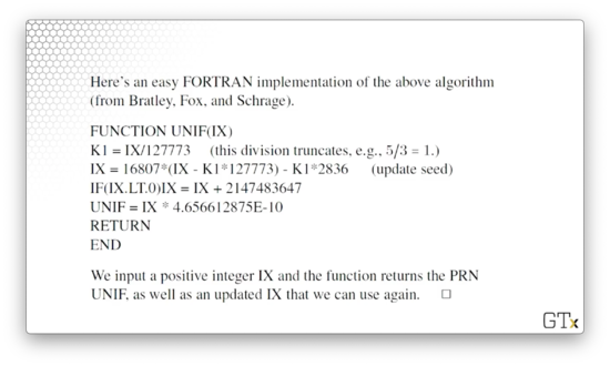
Alternatively, we can use an algorithm to generate pseudo-random numbers (PRNs); in other words, a series R1,R2,... of deterministic numbers that appear to be iid Unif(0,1). Pick a seed integer, X0, and calculate:
Xi=16087Xi−1mod231−1,i=1,2,...
Note that we saw this random number generator (RNG) in a previous lesson.
A given value of Xi exists on [0,231−1). To transform a given Xi into the corresponding Ri, which exists on [0,1), we use the following formula:
Ri=Xi/(231−1),i=1,2,...
Here is how we might program this RNG in Python:
# Tested with Python 3.8.3# I've done this with a generator. There is probably a better way. I am not a Python expert.defrng(seed): x_i = seedwhileTrue: x_i =16807* x_i %(2**31-1)yield x_i /(2**31-1)gen =rng(12345678)print(next(gen))# 0.621834785967057print(next(gen))# 0.17724774832709123print(next(gen))# 0.0029061334221186738print(next(gen))# 0.84338442554855print(next(gen))# 0.762040194478836
Alternatively, we can use this Fortran implementation.
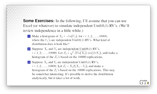
Exercises
Great Expectations
In this lesson, we are going to talk about computing the expected values of random variables. We are going to pay particular attention to something called LOTUS, which we will learn about soon.
Expected Value
The expected value (or mean), of a random variable, X is defined as:
E[X]={∑xxf(x) if X is discrete∫Rxf(x) if X is continuous
For discrete random variables, the expected value is the sum of xP(X=x) for all possible values of x. Likewise, for continuous random variables, the expected value is the integral of xf(x)dx over the real line, R.
In either case, we can think of the expected value as the weighted average of the possible values of X, where x is the value and f(x) is the weight given to that value.
Bernoulli (Discrete) Example
Suppose that X∼Bernoulli(p). Then, X=1 with probability p and X=0 with probability q=1−p. In other words,
X={1with prob. p0with prob. q=1−p
What is E[X]? Since X is a discrete random variable, we take the weighted average of the discrete values:
E[X]=x∑xf(x)=(1∗p)+(0∗q)=p
Uniform (Continuous) Example
Suppose that we have a random variable X∼Unif(a,b). This random variable has the following pdf:
f(x)={b−a1if a<x<b0otherwise
If this looks foreign to you, recall the example where we generated the pdf for X∼Unif(3,7)
If we integrate f(x) over R, we get E[X]. Note that we really only need to integrate over (a,b) because f(x) evaluates to 0 everywhere else:
E[X]=∫Rxf(x)dx
E[X]=0+∫abxf(x)dx+0
E[X]=∫abb−axdx
E[X]=b−a1∫abxdx
E[X]=b−a1(2x2)∣∣∣∣ab
E[X]=b−a1(2b2−2a2)
E[X]=b−a1(2b2−a2)
E[X]=2(b−a)b2−a2
E[X]=2(b−a)(b−a)(b+a)
E[X]=2(b+a)
This result makes sense. Given a random uniform sampling over a range (a,b), the expected value or weighted mean lies in the middle of the range: (a+b)/2.
Exponential (Continuous) Example
Suppose that we have a random variable, X∼Exponential(λ). This random variable has the following pdf:
f(x)={λe−λxif x>00otherwise
If we integrate f(x) over R, we get E[X]. Note that we really only need to integrate over (0,∞) because f(x) is undefined for x≤0:
E[X]=∫Rxf(x)dx=∫0∞xλe−λxdx=λ1
Computing this integral is left as an exercise to the reader. I am not typing out this whole thing.
Law of the Unconscious Statistician
Let's look at the Law of the Unconscious Statistician (LOTUS). This theorem gives us the expected value of some arbitrary function, h(X), applied to a random variable, X. In short,
E[h(X)]={∑xh(x)f(x) if X is discrete∫Rh(x)f(x) if X is continuous
The function h(X) can be anything "nice" (continuous? differentiable?), like h(X)=X2 or h(X)=1/X or h(X)=sin(X) or h(X)=ln(X).
Discrete Example
Suppose X is a discrete random variable with the following pmf:
f(x)=⎩⎪⎪⎪⎨⎪⎪⎪⎧0.3 if x=20.6 if x=30.1 if x=40 otherwise
Suppose we have a function h(X)=X3. We can calculate E[h(X)]=E[X3] as follows:
E[X3]=x∑x3f(x)=23(0.3)+33(0.6)+43(0.1)=25
Continuous Example
Suppose we have a random variable X∼Unif(0,2). X has the following pdf:
f(x)={0.50<x<20 otherwise
Suppose we have a function h(X)=Xn. We can calculate E[h(X)]=E[Xn] by integrating h(x)f(x)dx over the real line, although since we are dealing with a uniform distribution, we only need to integrate from 0 to 2:
E[Xn]=∫Rxnf(x)dx
E[Xn]=0+∫022xndx+0
E[Xn]=2(n+1)xn+1∣∣∣∣02
E[Xn]=2(n+1)2n+1−0
E[Xn]=n+12n
Moment, Variance, and Standard Deviation
Given a random variable, X, the expected value of X raised to the nth power, E[Xn], is the nth moment of X. Relatedly, the nth central moment of X is given as E[(X−E[X])n].
The variance of X is defined as the second central moment of X: Var(X)=E[(X−E[X])2]. From the equation, we can see that the variance of X is the expected value of the squared deviation of X from its mean.
Let's break it down from the inside out. E[X] is the expected value of X. X−E[X] captures how far the X tends to deviate from the mean. That deviation could be positive or negative, so we square it to make it positive. Finally, we take the average over all the squared deviances to compute the variance.
Whereas the expected value of X is a measure of the middle of the distribution, the variance of X measures the spread of the distribution.
With a little bit of algebra, we can come up with an alternative equation for the variance: Var(X)=E[X2]−(E[X])2.
The standard deviation of X is simply the positive square root of the variance of X.
Discrete Example
Suppose we have a random variable X∼Bernoulli(p). Recall that E[X]=p. Via LOTUS, we know that:
E[X2]=x∑x2f(x)=p
Given E[X2], we can calculate the variance of X:
Var(X)=E[X2]−E[X]2=p−p2=p(1−p)
Continuous Example
Suppose we have a random variable X∼Exp(λ). By LOTUS,
E[Xn]=∫0∞xnλe−λxdx=λnn!
Given E[Xn], we can calculate the variance of X using E[X2] and E[X]:
Var(X)=E[X2]−E[X]2=λ22−(λ1)2=λ21
Theorem
Let's consider the following theorem, which shows that expectation is a linear function. In other words:
E[aX+b]=aE[X]+b
Variance works slightly differently:
Var(aX+b)=a2Var(X)
Note that for variance, the b goes away, and this elimination makes sense. If we have a random variable and we shift if by some constant factor b, we haven't changed how much it is spread out, only where it is centered.
Example
Consider a random variable X∼Exp(3). Then:
E[−2X+7]=−2E[X]+7=−2∗31+7=319
Var(−2X+7)=(−2)2Var(X)=4∗91=94
Moment Generating Functions (Bonus)
Given a random variable, X, the moment generating function (mgf) of X is defined as MX(t)=E[etX]. Note that MX(t) is a function of t, not X.
Bernoulli Example
Consider a random variable X∼Bernoulli(p). Remember the pmf for X:
X={1with prob. p0with prob. q=1−p
We can use LOTUS to find MX(t):
MX(t)=E[etX]=x∑etxf(x)=et∗p+e0∗q=pet+q
Exponential Example
Consider a random variable X∼Exp(λ), which has a pdf f(x)=λe−λx,x>0. Again we can use LOTUS to find MX(t):
MX(t)=∫Retxf(x)dx
MX(t)=∫0∞etxλe−λxdx
MX(t)=λ∫0∞etxe−λxdx
MX(t)=λ∫0∞e(t−λ)xdx
MX(t)=λ−tλ, if λ>t
Note that if λ≤t, then the definite integral goes to infinity, so we have to set the constraint that λ>t.
Generating Moments (Theorem)
Why do we care about the moment generating function? Well, under certain technical assumptions, the kth moment of X is a function of the moment generating function. Specifically,
E[Xk]=dtkdkMx(t)∣∣∣∣t=0k=1,2,...
In other words, the kth moment of X is equal to the kth derivative of the mgf (with respect to t), evaluated at t=0.
Naturally, we name the moment generating function so because we can use it to generate moments!
Example
Consider a random variable X∼Exp(λ), which has an mgf MX(t)=λ/(λ−t),λ>t. Let's generate the first moment of X, which is just the expected value, E[X]:
E[X]=dtdMX(t)∣∣∣∣t=0
E[X]=dtdλ−tλ∣∣∣∣t=0
E[X]=(λ−t)2λ∣∣∣∣t=0
E[X]=λ2λ=λ1
Let's calculate the second moment of X, E[X2]:
E[X]=dt2d2MX(t)∣∣∣∣t=0
E[X]=dt2d2λ−tλ∣∣∣∣t=0
E[X]=dtd(λ−t)2λ∣∣∣∣t=0
E[X]=(λ−t)4λ∗2(λ−t)∣∣∣∣t=0
E[X]=(λ−t)32λ∣∣∣∣t=0
E[X]=λ32λ=λ22
Given the second moment of X, we can calculate the variance of X:
Var(X)=E[X2]−(E[X])2=λ22−λ21=λ21
Functions of a Random Variable
In this lesson, we will explore functions of random variables. In particular, we will focus on how functions change the distribution of the underlying random variable. This analysis has huge implications for the course, especially regarding random variate generation.
Problem
Suppose we have a random variable, X, and we know the pmf/pdf, f(x). Now, let's look at a new random variable, which is a function of X, Y=h(X). Our task is to find g(y), the pmf/pdf of Y.
Here are some basic examples, which we won't prove now:
If U∼Unif(0,1), then Y=−ln(U)/λ∼Exp(λ). We have seen this transformation before.
Discrete Example
Let X denote the number of heads seen from two coin tosses. We know that X has the following pmf, f(x):
f(x)=⎩⎪⎨⎪⎧1/4, if x=01/2, if x=11/4, if x=2
How do we compute the pmf, g(y), for Y=X3−X? Let's map x to y:
y=x3−x=⎩⎪⎨⎪⎧0, if x=00, if x=16, if x=2
With this correspondence between x and y, we can now relate f(x) to g(y). For example, g(0)=P(Y=0)=P(X=0)+P(X=1)=3/4. Similarly, g(6)=P(Y=6)=P(X=2)=1/4. Thus, we have the pmf for Y:
g(y)={3/4, if y=01/4, if y=6
Continuous Example
Suppose a random variable X has a pdf f(x)=∣x∣,−1≤x≤1. Find the pdf of Y=X2.
First, let's find the cdf of Y, G(y). Remember that, for a given value of y, the cdf at y is equal to the pdf of all Y≤y. In other words:
G(y)=P(Y≤y)
Let's substitute X2=Y:
G(y)=P(X2≤y)
Note that we only know about X, not X2, so we take the square root, and rearrange the inequality:
G(y)=P(−y≤X≤y)
By definition, this probability equals the integral of the pdf of X between these two bounds, so we integrate.
G(y)=∫−yy∣x∣dx
G(y)=∫−y0−xdx+∫0yxdx
G(y)=2−x2∣∣∣∣−y0+2x2∣∣∣∣0y
G(y)=0+2y+2y−0=y,0<y<1
Note that since x is constrained to [−1,1], y=x2 is constrained to (0,1).
Remember, the pdf is the derivative of the cdf: g(y)=G′(y)=1. Note that because of the constraint on y:
g(y)={1,0<y<10,otherwise
This pdf, which should look familiar, describes the random variable Y∼Unif(0,1).
Inverse Transform Method
Let's suppose that X is a continuous random variable with cdf F(x). Then, amazingly, the random variableF(X) is a Unif(0,1) random variable: F(X)∼Unif(0,1).
Proof
Let Y=F(X). Then the cdf of Y is, by definition:
P(Y≤y)
Let's plug in what Y equals:
P(Y≤y)=P(F(X)≤y)
We only know about X, not F(X). Let's apply F−1 to both sides of the inequality to free up the X:
We have just shown that the cdf of Y=F(X) is equal to y. The pdf, given that cdf, is 1, which is the pdf for a Unif(0,1) random variable. Thus, F(X)∼Unif(0,1).
Exponential Example
Let's do a simple example to show we can generate random variables. In particular, we want to generate X∼Exp(λ), and we are going to use the inverse transform method to do this.
Suppose that X∼Exp(λ), with cdf F(x)=1−e−λx,x≥0. The inverse transform theorem implies that:
F(X)=1−e−λX∼Unif(0,1)
Let U∼Unif(0,1). Since F(X) is uniform, we can set F(X)=U. Now, we can solve for X:
F(X)=1−e−λX=U
1−e−λX=U
1−U=e−λXU
ln(1−U)=−λX
λ−ln(1−U)=X∼Exp(λ)
Again, we have just demonstrated how we can transform a random variable from one distribution, U∼Unif(0,1), into a random variable from another distribution: X∼Exp(λ).
For instance λ=2 and U=0.27, then X=0.157 is an Exp(2) realization.
Weibull Example
Suppose we have a random variable X with the Weibull distribution. X has the following cdf:
F(x)=1−e−(λx)B,x>0
Note that if we set B=1, we have the cdf for X∼Exp as a special case.
Under the inverse transform method, we can set F(X)=U and then solve for X:
U=1−e−(λX)B
1−U=e−(λX)B
ln(1−U)=−(λX)B
[ln(1−U)]1/B=−λX
X=λ1[ln(1−U)]1/B
Bonus Theorem
Here's another way to get the pdf of Y=h(X) for some continuous function h. The cdf of Y is:
FY(y)=P(Y≤y)=P(h(X)≤y)=P(X≤h−1(y))
Remember, FX(x)=P(X≤x). Correspondingly, P(X≤h−1(y))=FX(h−1(y)). In other words,
fY(y)=dydFY(y)=dydFX(h−1(y))
Taking advantage of the fact that the derivative of the cdf is the pdf, we can compute the derivative using the chain rule:
dydFX(h−1(y))=fX(h−1(y))∣∣∣∣dydh−1(y)∣∣∣∣
Since the pdf has to be greater than or equal to zero, we have to take the absolute value of the derivative of h−1(y). That way, the product of the two terms is always 0 or positive.
Armed with this result, we can prove LOTUS. Remember the definition for the expected value of a random variable, Y:
E[Y]=∫RyfYdy
Remember, we have an expression for fY:
fY(y)=fX(h−1(y))∣∣∣∣dydh−1(y)∣∣∣∣
Thus:
E[Y]=∫RyfX(h−1(y))∣∣∣∣dydh−1(y)∣∣∣∣dy
Take it on faith that this expression simplifies to:
E[Y]=∫RyfX(h−1(y))dh−1(y)
If we set x=h−1(y), then you get LOTUS:
E[Y]=∫Rh(x)fX(x)dx
Jointly Distributed Random Variables
In this lesson, we will review two-dimensional random variables that may or may not be correlated with each other. As a basic example, think height and weight!
In simulation, we might be concerned with consecutive correlated waiting times. If we have customers in a line, then obviously the waiting times between customers will be correlated with each other.
Joint and Marginal CDF
Let's consider two random variables, X and Y, interacting together - think height and weight. We can define the joint cdf of X and Y as:
F(x,y)≡P(X≤x,Y≤y),for all x,y
The marginal cdf of X is the cdf of X, regardless of Y: FX(x)=F(x,∞). Similarly, the marginal cdf of Y is FY(y)=F(∞,y).
Let's consider the marginal cdf in the context of height in inches (X) and weight in pounds (Y). Say we want to compute F(72,∞). This expression describes the probability of sampling an observation with a height less than 72 inches and a weight less than ∞. However, we know that every observation must have a weight less than ∞ by the definition of a cdf. As a result, we essentially are removing Y from consideration and focusing just on X.
Joint PMF
If X and Y are discrete random variables, then the joint pmf of X and Y is f(x,y)≡P(X=x,Y=y). Of course, the sum of the pmf over all x and y is equal to 1: ∑x∑yf(x,y)=1.
Just as we computed the marginal cdf of X and Y, we can also compute the marginal pmf of X and Y. The marginal pmf of X is fX(x)=P(X=x)=∑yf(x,y). Similarly, the marginal pmf of Y is fY(y)=P(Y=y)=∑xf(x,y). In either case, we fix one of the two random variables at a certain value and then sum the probabilities over all values of the other random variable at that value.
Example
Consider the following table, with gives the joint pmf, f(x,y) along with the accompanying marginal pmfs, fX(x) and fY(y) for two random variables, X and Y:
The possible values for X are 2, 3, and 4, and the possible values of Y are 4 and 6. The numbers in the interior of the table give the joint pmf for the corresponding (Y=y,X=x) pair. For example, f(X=2,Y=4)=0.3, the upper-leftmost cell in the interior. If we add the interior entries, we get 1: ∑x∑yf(x,y)=1.
Let's look at the marginal pmf for X, fX(x). For X=2, fX(2)=∑yf(2,y). If we expand out the sum, we get fX(2)=f(2,4)+f(2,6)=0.3+0.1=0.4. We can apply similar sums to compute fX(3) and fX(4). Of course, ∑xfX(x)=1.
Let's look at the marginal pmf for Y, fY(y). For Y=4, fY(4)=∑xf(x,4). If we expand out the sum, we get fY(4)=f(2,4)+f(3,4)+f(4,4)=0.3+0.2+0.1=0.6. We can apply the same logic to compute fY(6). Of course, ∑yfY(y)=1.
Joint PDF
If X and Y are continuous, then the joint pdf of X and Y is the second partial derivative of the cdf: f(x,y)≡∂2/∂x∂yF(x,y). Note that if we take the double integral of the pdf over the real line, we get 1, as per the definition of the pdf: ∫R∫Rf(x,y)dxdy=1. Note that since our pdf is two-dimensional, we need to integrate in both dimensions to sum the probabilities for all possible (x,y) pairs.
Just as we saw with the marginal pmfs previously, we can calculate the marginal pdfs of X and Y as:
fX(x)=∫Rf(x,y)dy,fY(y)=∫Rf(x,y)dx
Note that this construction matches the marginal pmf for the discrete variables. The marginal pdf for X, fX(x) equals the sum of the probabilities of f(x,y), over all values of y. Similarly, the marginal pdf for Y, fY(y) equals the sum of the probabilities of f(x,y), over all values of x.
Example
Suppose we have two random variables, X and Y, whose joint pdf is the following:
f(x,y)=421x2y,x2≤y≤1
Note the limits of x and y: x2≤y≤1. Limits like these have ramifications when it comes to independence, which we are going to talk about shortly.
Let's take a look at the marginal pdfs, fX(x) and fY(y). First, fX(x):
fX(x)=∫Rf(x,y)dy
Note that, since we are integrating with respect to y, the limits of integration become the limits of y. In other words, we integrate from x2 to 1:
fX(x)=∫x21421x2ydy
Now, since we are integrating with respect to y, the expression 21x2/4 is a constant, which can move outside the integral:
fX(x)=421x2∫x21ydy
Let's complete the integration:
fX(x)=421x22y2∣∣∣∣x21
fX(x)=421x2(21−2x4)
fX(x)=821x2(1−x4)
Note that since x2≤y≤1, fX(x) is only defined for −1≤x≤1. If ∣x∣>1, then x2>1>y, which breaks the inequality.
Now, let's find fY(y):
fY(y)=∫Rf(x,y)dx
Note that, since we are integrating with respect to x, the limits of integration become the limits of x. In other words, since x2≤y, then −y≤x≤y, which become our new limits of integration:
fY(y)=∫−yy421x2ydx
Because we are integrating with respect to x, the expression 21y/4 is a constant, which can move outside the integral:
fY(y)=421y∫−yyx2dx
Let's complete the integration:
fY(y)=421y3x3∣∣∣∣−yy
fY(y)=421y(3(y)3−3(−y)3)
fY(y)=421y(3y3/2+3y3/2)
fY(y)=421y(32y3/2)
fY(y)=1242y5/2=27y5/2
Remember the limits: x2≤y≤1. Since x2 cannot be negative, and y cannot be greater than one, fY(y) is only defined for 0≤y≤1.
Independence
Random variables X and Y are independent if f(x,y)=fX(x)fY(y) for all x,y. Consider the following theorem: X and Y are independent if we can write their joint pdf as f(x,y)=a(x)b(y) for some functions a(x) and b(y)andx and y don't have funny limits (their domains don't depend on each other).
Examples
If f(x,y)=cxy for 0≤x≤2,0≤y≤3, then X and Y are independent. How can we tell? First of all, if a(x)=cx and b(y)=y then f(x,y)=a(x)b(y). Second, we don't have any funny limits; that is, x and y don't depend on each other.
Let's revisit the pdf f(x)=21x2y/4, for x2≤y≤1. In this case, X and Y are not independent. How can we tell? First of all, if a(x)=21x2/4 and b(y)=y, then f(x,y)=a(x)b(y). However, we do have funny limits: x2≤y≤1 indicates that x constrains y, and vice versa.
As a final example, consider f(x,y)=c/(x+y) for 1≤x≤2,1≤y≤3. In this case, X and Y are not independent. Even though we don't have any funny limits, there are no a(x) and b(y), such that f(x,y)=a(x)b(y).
Conditional PDF/PMF
The conditional pdf (or pmf) of Y given X=x is f(y∣x)≡f(x,y)/fX(x), assuming fX(x)>0. This is a legit pdf/pmf. For example, in the continuous case, ∫Rf(y∣x)dy=1, for any x.
Example
For example, suppose f(x,y)=21x2y/4 for x2≤y≤1. We can calculate f(y∣x) using f(x) and fX(x), which we calculated previously:
f(y∣x)=fX(x)f(x,y)
f(y∣x)=821x2(1−x4)421x2y
f(y∣x)=821(1−x4)421y
f(y∣x)=821421(1−x4)y
f(y∣x)=1−x42y,x2≤y≤1
Note that the final equation contains both the variables x and y. We are querying about y, and we have information about x - that's the whole "given x" part of the conditional - so the presence of the two variables makes sense.
Theorem
If X and Y are independent, then f(y∣x)=fY(y) for all x,y. In other words, information about X contributes nothing to the distribution of Y. For example, let X equal the current IBM stock price, and Y equal the current temperature on Mars. The information Y=30∘ gives us no information regarding IBM stock.
Let's prove this theorem. Remember the formula for the conditional pdf, f(y∣x):
f(y∣x)=fX(x)f(x,y)
Remember that if X and Y are independent, then f(x,y)=fX(x)fY(y). So:
f(y∣x)=fX(x)fX(x)fY(y)=fY(y).□
Conditional Expectation
If we can compute the conditional pdf/pmf f(y∣x), then we can compute the conditional expection of Y given X=x as the following:
Conditional expectation is very important as it allows us to update our expectation about Y given information about X. For example, suppose that we have a person who is seven feet tall, and we are interested in his expected weight: E[Y∣X=7]. The information that he is seven feet tall will give us an expected value for his weight that is probably going to be greater than the expected weight of some random person, about whom we have no height information: E[Y].
Example
Let f(x,y)=21x2y/4, if x2≤y≤1. Then:
E[Y∣X]=∫Ryf(y∣x)dy
E[Y∣X]=∫x211−x42y2dy
E[Y∣X]=1−x42∫x21y2dy
E[Y∣X]=1−x42(3y3∣∣∣∣x21)
E[Y∣X]=1−x42(313−3x6)=32×1−x41−x6
Note that the conditional expectation is a function of x, which makes sense: prior information about x changes the expected value of Y, and the degree to which this information updates the expected value is a function of x.
OMSCS Notes is made with
in NYC by Matt Schlenker.