Simulation
Arena
37 minute read
Notice a tyop typo? Please submit an issue or open a PR.
Arena
Process-Interaction Overview
In this lesson, we will quickly review the process-interaction approach that Arena uses.
Process Interaction
In the process interaction method, we consider generic customers and the sequence of events and activities they undergo as they move through the system. In Arena, which takes the process interaction worldview, we call the customers entities and the events processes, and we say that entities move through processes.
At any given time, the system may contain many of these generic entities interacting with one another. For example, two entities might be trying to interact with the same process, which might be a single server. In this case, one entity receives service while the other waits in line. Arena oversees all the entities and observes how they move through the system and compete with each other for access to processes.
The entities flow through a network of modules (blocks) that describe their behavior, and we can represent this network using a process flowchart.
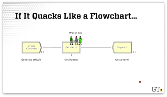
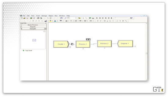
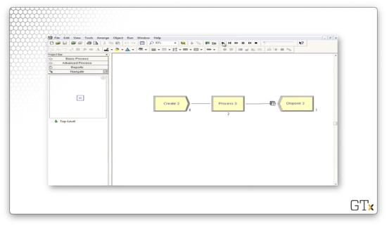
For example, let's suppose that people show up at the barbershop, they get served, potentially after waiting in line, and then they leave. In Arena, we generate the arrival using the Create module. We interact with the barber using the Process module. We remove the entity from the system with the Dispose module.
Here is a flowchart representing the barbershop simulation we just described. We can see that we have generated sixty-two entity arrivals so far. Four of the entities are inside the process, either being served or waiting in the queue, and fifty-eight have left the system.
Let's Meet Arena
In this lesson, we will finally start looking at Arena. First, we'll talk about how to get the software, and then we'll look at some of the functionality.
Getting Arena
We can download and install the free student version of Arena here. For better or worse, this application only runs on Windows machines. If we aren't using Windows, we can access Arena via the Georgia Tech virtual labs. Alternatively, we can download and boot Windows in a virtual machine and then run Arena "locally".
Introducing Arena
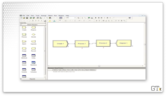
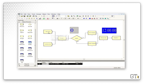
Let's take a look at the main Arena screen.
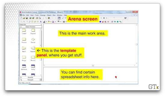
We have the main work area, where we will drag, drop, and connect items from the sidebar on the left. That sidebar is the template panel, and it holds most of the building blocks for our simulations. Finally, the bottom pane displays certain runtime and spreadsheet information that is occasionally useful.
The main menu toolbar has several features.
The File menu provides the usual new, open, close, and save functionality, but it also lets us import different template panels and background pictures. As it turns out, there are many Arena template panels that enhance the package's basic capabilities, and we can import those from this menu.
The Edit menu allows us to edit various things as well as insert objects. The View menu lets us see different toolbars and customize our named views, which are essentially saved screens we can load on demand.
The Tools menu exposes some cool features. We can use the Input Analyzer to fit distributions, OptQuest to run certain optimizations, and AVI capture to record simulation runs for sharing.
The Arrange, Object, and Window menus provide some visualization tools and aids that we can use to present things more nicely from a visual perspective.
We use the Run menu to set up a simulation and execute it however we want. We can speed up simulations, slow them down, advance them frame by frame, pause them, stop them, and more.
Let's look at the basic process template panel again.
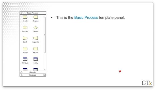
This panel contains the basic building blocks that we can use to set up some simple simulations. We have already briefly talked about some of these modules, such as create, process, and dispose. We drag these modules over to the main work area to make our models.
There is a second set of icons below these blocks that are related to spreadsheets. For example, "Entity" keeps track of customers, and "Attributes" keeps track of different properties of the customers.
DEMO
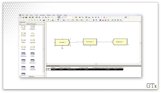
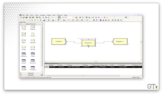
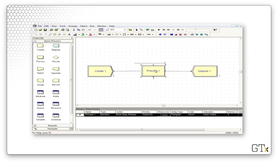
In this demo, we are going to build a simple queueing model. To do so, we will drag and drop the Create, Process, and Dispose modules and connect them appropriately.
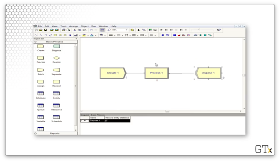
When we run the simulation, we see customers being created, moving through a self-service process, and then exiting the system.
Note that we can use the navigation toolbar to pause the simulation or step forward one event at a time. Of course, we can also stop the simulation completely.
In later lessons, we will customize the modules to meet more specific modeling needs. For right now, here is a basic preview of the customization options for the Create module.
By default, customer interarrival times are generated according to an exponential distribution with a mean of one hour.
Let's look at some options for the Process module.
Here we see that the self-service delay is modeled by a triangular distribution, which is parameterized by a minimum, mode, and maximum value of 0.5, 1, and 1.5 hours, respectively.
Basic Process Template
In this lesson, we will look at the basic process template in more detail. We'll be able to use the items from this template to make our initial simulations: all we have to do, essentially, is drag and drop.
Modules
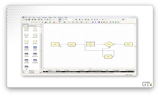
The top half of the process panel contains the modules that we drag into the main workspace area. These modules are the building blocks that "do stuff" in our simulation. We connect these modules to form a flowchart representation for our simulation model.
As we saw, we use the Create module to generate arrivals, and we use the Dispose module to remove customers from the system. We use the Process module to have customers interact with servers and potentially wait in line.
We drag these modules over to the workspace area, build the flowchart, fill in some numbers, hit the go button, and run our simulation.
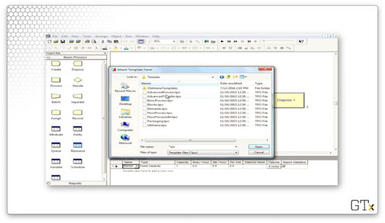
Suppose we are interested in more advanced modules than those that come in the basic template panel. In this case, we can go to File > Template Panel > Attach and browse for more interesting templates.
Spreadsheets
The bottom half of the process panel contains spreadsheets that give us both information and the capability to change certain system parameters - the number of servers or the service rate, perhaps.
For example, the Variable spreadsheet defines global quantities. We might maintain a WIP (work in process) variable that gets updated as the simulation progresses. As a customer shows up, we increment WIP. As a customer leaves, we decrement WIP. We could track the value of WIP in this spreadsheet.
The Resource spreadsheet keeps track of the names and capacities of the different servers. We can change the capacities in this spreadsheet, or we can look at the Schedule spreadsheet to schedule capacity changes over time.
DEMO
Let's look at a demo of the basic process template. First, we'll talk about a couple of features, and then we'll look at how we get other templates.
Let's refresh on the simulation that we built last time. Customers are created every once in a while, they pass through a self-service process, and then they are disposed.
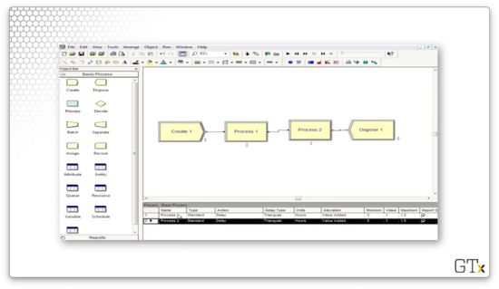
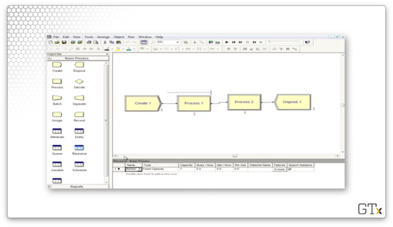
We can add another process to the model. Notice that we keep track of both processes in the bottom panel.
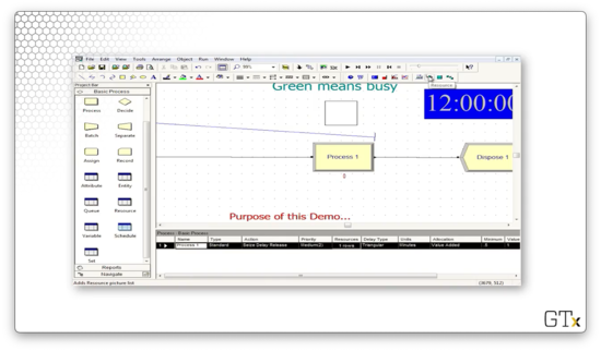
If we click on the Resource spreadsheet, we see that we have no resources in the system.
Let's create one. We can change our process from a "Delay" action - the self-service we've been looking at so far - to a "Seize Delay Release" action.
We add a resource, which we will call "Barber".
If we go back to the Resource spreadsheet, we can see that we have a "Barber" resource.
Now we can run the simulation and watch customers queue up while they wait for the barber.
Let's look at how we might load more advanced templates. We first go to File > Template Panel > Attach. From here, we can browse to C://Program Files/Rockwell Software/Arena/Template or a similar location. Once there, we can select any of the templates to import.
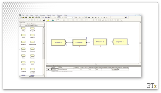
After importing a new template, we can see that we have access to many new modules we didn't see before, such as Delay and Seize.
Create, Process, Dispose Modules
In this lesson, we'll discuss the Create, Process, and Dispose modules found in the basic template panel, and then we'll build our first official simulation.
Create-Process-Dispose
In the Create module, we periodically generate customer arrivals. In the Process module, we perform work on customers, potentially after a waiting period. In the Dispose module - known as "Terminate" in GPSS and "Send to Die" in Automod - we remove customers from the system.
How to Use
We drag and drop modules from the template panel to the main work area, where they usually connect to one another automatically. Note that customers traverse connections instantaneously; there is no space between modules that delays customer movement. We can program in certain travel times, but we aren't doing that quite yet. After we connect our modules, we start the simulation and observe customers moving through the system.
Deeper Dive into Create
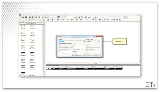
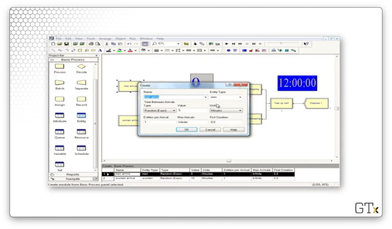
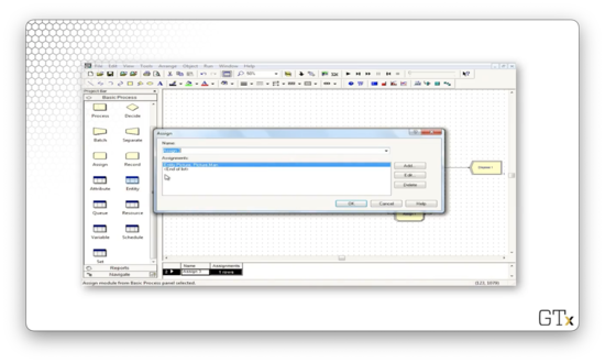
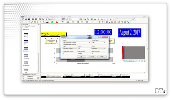
We can click into the modules and see the various configuration options. Let's dive deeper into the Create module.

We can edit the name of the module, which is displayed in the main work area when running the simulation. We occasionally need to refer to a module by its name, so we should choose it wisely. Note that we can't give two modules the same name.
We edit the type of entity. In this case, the entity defaults to "Entity 1", but we might want to name it something like "Barber Customers" in light of our recent demos.
We can also specify the interarrival distribution. In this case, the "Random (Expo)" signifies that we are generating interarrival times from an exponential distribution. Correspondingly, we have fields for the mean of the distribution (one) and the units for the values sampled from the distribution (hours).
Below the interarrival configuration, we can specify the number of customers per arrival. Here we have a value of one, but we might change this if we are simulating a restaurant or some other system where people arrive in groups.
Additionally, we can specify the maximum number of allowed arrivals. Sometimes, we want to end the simulation after a particular number of people arrive, but here, we are allowing infinite arrivals.
Finally, we can specify the first creation time. In this simulation, a customer is waiting at the door and arrives right at time zero, but we can set the first arrival to some later time if we want.
Process and Dispose Modules
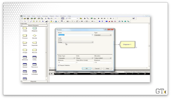
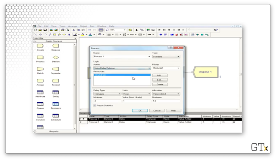
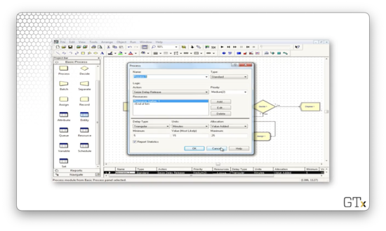
Let's look at the Process module.
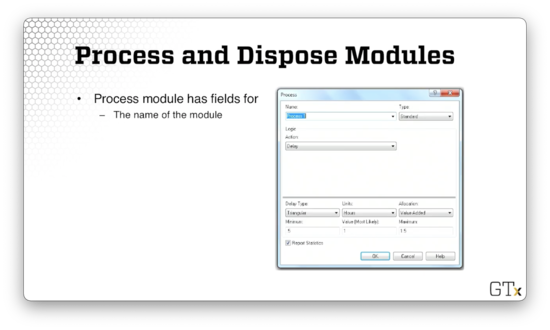
Just like the Create module, we can specify the name of the module.
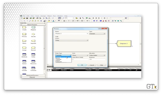
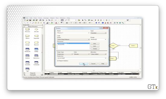
We can also specify the type of action. For example, we can try to reserve a resource or free a resource in use. A "delay" action refers to a self-service process, whereas a "seize, delay, release" action involves acquiring a resource, receiving service, and then releasing that resource to serve another entity.
We can also specify how long we want the customer to be delayed while being processed: the service time. In this case, we have service times sampled from a triangular distribution, with a minimum, mode, and a maximum of 0.5, 1, and 1.5 hours, respectively.
In the Dispose module, we get rid of entities. There isn't much to configure with this module outside of the name.
DEMO
In this demo, we'll look at different settings for the Create, Process, and Dispose trio of modules.
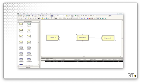
Let's create our favorites simulation: a Create module connected to a Process module connected to a Dispose module.
Let's see how we might configure the Create module. For example, instead of generating interarrival times from an exponential distribution, we could have customers arrive at a constant rate.
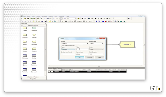
Here we have specified that we want one customer to arrive every hour. We could change the units so that customers arrive once every minute or second.
Alternatively, we could have customers arrive according to a custom expression. For example, we could specify that we want interarrival times generated from a Uniform(2,4) distribution.

We could get even fancier. Perhaps we want to generate arrivals according to the product of a Uniform(2,4) random variable and a Normal(3,0.5) random variable. We can specify that using the UNIF(2,4) * NORM(3, 0.5) expression.
Similarly, we can customize the number of entities per arrival. We can either enter a whole number or a distribution. For example, if we want arrival sizes to be generated from a Poisson distribution, we can use the following expression: POIS(3).
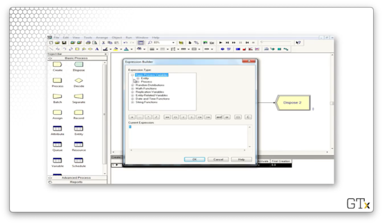
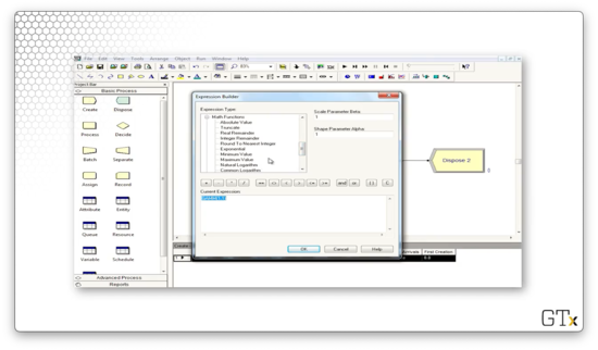
If we want even more complicated logic, we can right-click and select Build Expression. Here, we have a whole host of building blocks for creating mathematical expressions of arbitrary complexity.
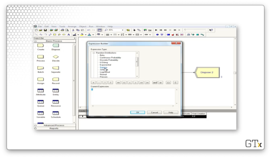
For example, we can build expressions using different probability distributions.
We can insert various math functions.
Let's look now at the Process module. We can select different distributions from which to sample service times, and we can change the units as appropriate.
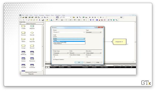
We can also change the action type. The default is "Delay", but we can also select "Seize Delay", "Seize Delay Release", and "Delay Release".
If we accidentally delete a connection between two modules, we can click on the "Connect" button on the main toolbar to rejoin them.
Details on the Process Module
In this lesson, we will learn more about the various options inside the Process module. This module allows us to grab servers, use them, and then release them for the next entity to use. Along the way, the module automatically sets up and manages a queue if we need one.
Seize-Delay-Release
Here are some of the different actions we can select in the Process module.
We can take a simple "Delay" action, where we delay ourselves while we self-serve. This type of action doesn't require any resources.
We can also take a "Seize-Delay-Release" action. In this action, we grab a resource (server), spend time getting served, and then free the server for the next entity to use. If we try to seize a resource that isn't available, we may have to wait in a queue.
We can also take a "Seize-Delay" action. Here, we grab at least one resource and spend time receiving service. If we take this action, we have to remember to manually release the resource at a later time, or else a giant line will form.
When might we seize and delay with no corresponding release? Suppose we are modeling patient flow in a hospital. A patient might seize a room and occupy it for some time. When they leave, we might have to clean the room before the next patient can seize it. Thus, we would have to manually release the room after the intermittent process of cleaning it.
Similarly, we might take a "Delay-Release" action. In this action, we use a previously seized server for a while and then free him for the next customer to use.
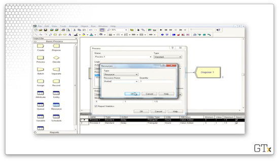
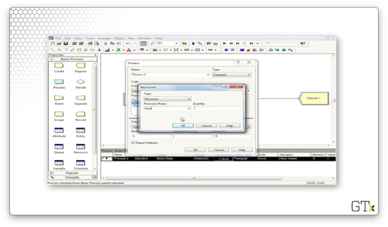
Resource Dialog Box
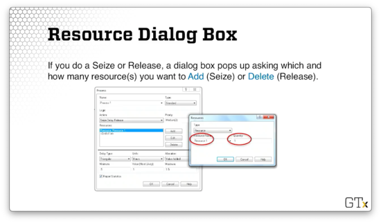
If we are performing an action that involves a Seize or Release, we will see a dialog box pop up asking us how many resources we want to add (Seize) or delete (Release).
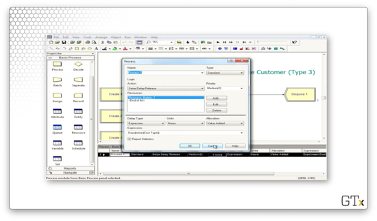
Here we can see that we have chosen the "Seize Delay Release" action, and we see the corresponding popup asking us which resource we want to add and how many we need to seize. In this case, we see that we want one of "Resource 1".
As a more concrete example, let's revisit the barbershop scenario from before. Suppose that a customer enters the Process module and executes a Seize-Delay-Release to grab and use one unit of the barber resource. We can specify both the type of resource and the quantity in the dialog box.
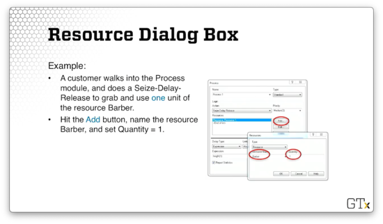
By default, the Process is given the name "Process 1". The Process includes the resource and the default queue, which is named "Process 1.Queue". As soon as we perform a "Seize-Delay-Release" of the barber, this queue automatically forms.
Let's look at a slightly different example. Suppose that every customer uses two barbers instead of one. In this case, we set the number of barbers to two instead of one when adding the resource.
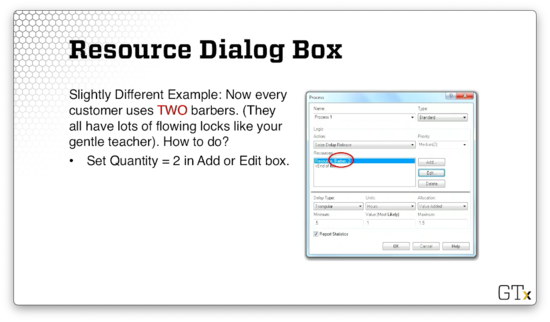
Note the distinction between the number of barbers in the store and the number of barbers required by a customer. For example, there may be five barbers in the store, and each customer needs precisely two of them. We are dealing with the two barbers per customer piece in this lesson. Later, we will look at the Resource spreadsheet and see how to set the capacity of the barber resource to five.
DEMO
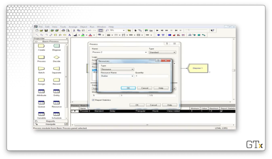
In this demo, we will look at different issues involving the Process module. As before, we will set up our Create, Process, and Dispose module connections.
By default, we are only performing a Delay action in the Process module. Let's change that action to Seize-Delay-Release. Since we are seizing a resource, we have to specify that resource; in this case, we will grab a single barber.
When we run the simulation now, we see the customers lining up in the queue while waiting for the barber to be freed.
Let's change the action from Seize-Delay-Release to just Seize-Delay. As we said before, the queue will grow steadily if we don't release our resources after use.
Let's fix this problem by adding another Process module with a Delay-Release action. What resource do we want to release? The barber that we previously seized, of course. We don't really care about this Process's delay, so we can decrease it to virtually nothing.
Let's see if this approach fixes the queueing bottleneck in our simulation.
Remember that we said that we could also seize multiple resources. Let's edit our first Process block to seize a manicurist alongside the barber. We will also change the action from Seize-Delay to Seize-Delay-Release.
In this case, we can grab as many resources as we need without changing the simulation dynamics. Of course, if the resources were available according to different schedules - this is not the case here - then the dynamics could change drastically.
Deadlock DEMO
Let's look at an example of a deadlock.
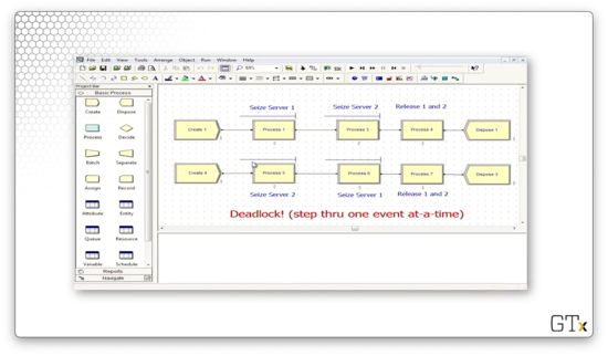
In this example, we create two separate streams of arrivals. Customers arriving from the first stream perform a Seize-Delay on resource one, followed by a Seize-Delay on resource two, and finally a Delay-Release on both resources.
Meanwhile, customers arriving from the second stream seize resources in the opposite order. First, they perform a Seize-Delay on resource two, followed by a Seize-Delay on resource one, followed by a Delay-Release on both resources.
Let's move through this simulation one step at a time. A customer first arrives from stream one and seizes resource one. Next, a customer arrives via stream two and seizes resource two. Another customer arrives via stream two and queues behind the first customer. A second customer arrives from stream one and queues behind the first customer of that queue.
Customer one from stream one leaves service from resource one and tries to seize resource two. However, this customer cannot acquire resource two because the first customer from stream two currently holds that resource. When that customer finishes being served by resource one, he goes to wait in line to receive service from resource two.
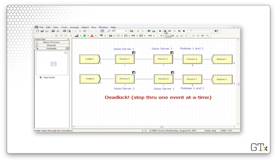
At this point, everything grinds to a halt. No resources can be released before additional resources are acquired. However, those resources cannot be acquired because the customers who have seized them haven't had the opportunity to release them.

Resource, Schedule, Queue Spreadsheets
In this lesson, we will shift our focus from modules to spreadsheets. We use spreadsheets to change the properties of various components involved in the simulation, such as resource capacities and queue characteristics.
Resource Spreadsheet
We can click on the Resource spreadsheet, found in the basic template panel, to see a list of the current model's resources, which displays at the bottom of the screen.
For example, in the image below, we see two resources, a barber and a pedicurist. The barber has a fixed capacity of four, and the pedicurist has a fixed capacity of one.
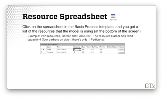
Remember that capacity refers to the number of a resource's servers on duty, not necessarily the number of servers that the customer requests. For example, there may be four barbers on the floor, but we usually only need one barber to give us a haircut.
We usually regard a resource's servers as identical and interchangeable. If the servers are different, we have to handle them not as a single resource but rather as a resource set.
Resources are automatically sent to the spreadsheet when we define them in the Process module. Alternatively, we can generate a new resource from the Resource spreadsheet directly.
We can also change the fixed capacity to a schedule, which means that the resource's capacity varies over time. For example, workers often take breaks, at which point they don't provide service for a short while, and we can use a schedule to reflect that.
Schedule Spreadsheet
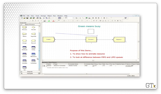
We set schedules for servers using the Schedule spreadsheet. We can go to the Resource spreadsheet and change the Type field from "Fixed Capacity" to "Based on Schedule".
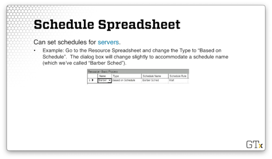
In this example, we've associated a schedule called "Barber Sched" with the barber resource. If we head over to the Schedule spreadsheet, we will see that Arena has created this schedule for us.
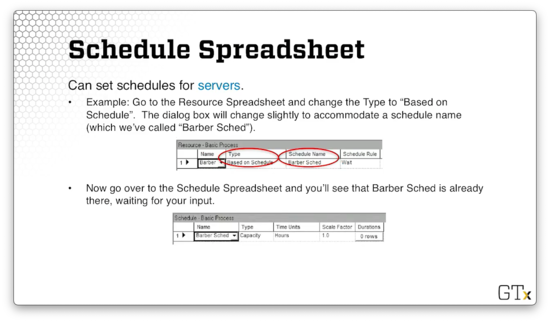
This schedule is a capacity schedule, which means that it varies the capacity of a resource over time. We can describe the schedule by adding entries in the "Durations" column. This column lets us declare how many servers are on duty at different points throughout the scheduling period.
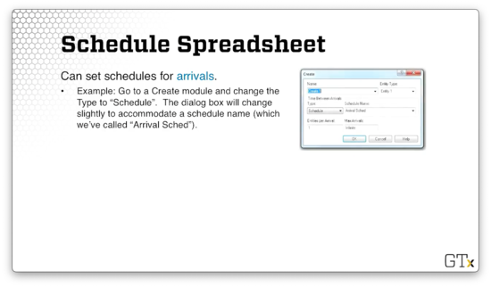
We also set schedules for arrivals. Arrivals change throughout the day; not everyone shows up to the Waffle House at the same rate hour over hour. We can go to the Create module and change the Type to "Schedule".
In this example, we've associated the arrivals with a schedule, instead of a distribution, called "Arrival Sched". Again, if we head over to the Schedule spreadsheet, we will see that Arena has created this schedule for us.
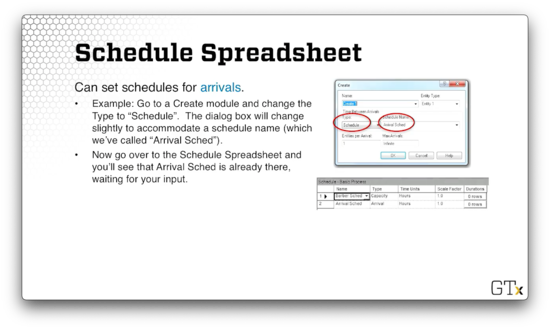
This schedule is not a capacity schedule because it has nothing to do with resources. Instead, it's an arrival schedule: it schedules arrivals.
DEMO
In this demo, we will focus on the series of spreadsheets we discussed in the previous lesson. We will start with our favorite Create, Process, and Dispose setup.
In the Create module, we sample interarrival times from an exponential distribution with a mean of 0.5 hours. In the Process module, we perform a Seize-Delay-Release on a single barber. We sample service times from a triangular distribution with a most-likely value of one hour. Because of this disparity between arrivals and service, the queue grows unbounded.
Let's head over to the Resource spreadsheet and see if we can provide this barber with some relief. As we can see, the barber resource currently has a capacity of one.
If we change the capacity to two, we see that the queue never grows to more than a few people.
As we mentioned, we can schedule the capacity of resources instead of using a fixed capacity. Let's change the Type column to "Based on Schedule" and enter "Barber Sched" into the Schedule Name column.
If we go over to the Schedule spreadsheet, we see our new schedule.
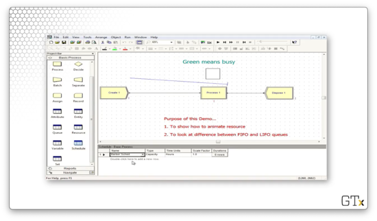
If we click into the "Durations" column, we see a time plot where we can declare the resource's capacity at each time slice.
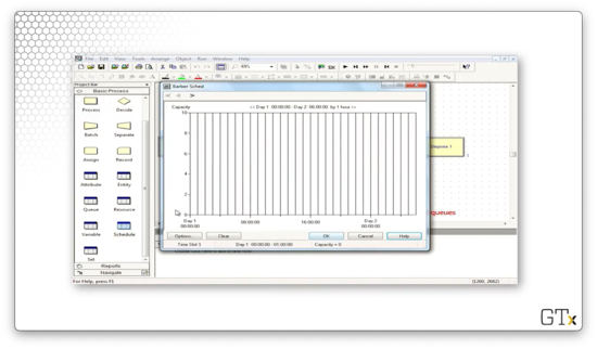
Let's schedule one server for the first hour of the simulation, two servers for the second hour, zero servers for the third hour, and four servers for the fourth hour.
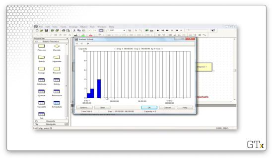
As we might expect, the line will grow throughout the first hour. During hour two, the two servers will hopefully be able to consume the queue. In hour three, the queue will grow unbounded, but, hopefully, in hour four, the four servers can bring it back down to a manageable size.
We can visualize time more easily if we create a clock by clicking on the clock icon in the toolbar.
At the end of the first hour, we have fifty people in the queue.
At the end of the second hour, we have brought the queue down to forty customers.
At the end of hour three, the queue has 172 customers.
Finally, after hour four, our four servers have brought the queue back down to 43 customers.
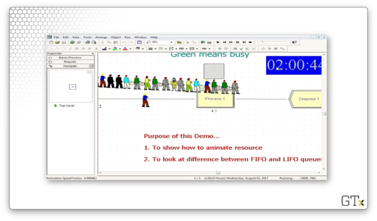
What happens next is that the schedule repeats itself, so we see the same resource capacities over the next four hours that we saw over the previous four.
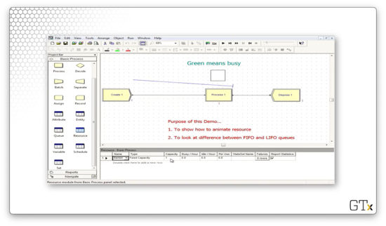
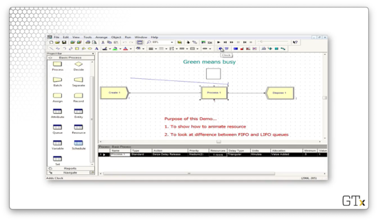
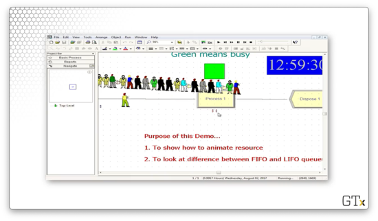
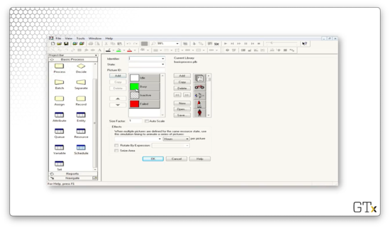
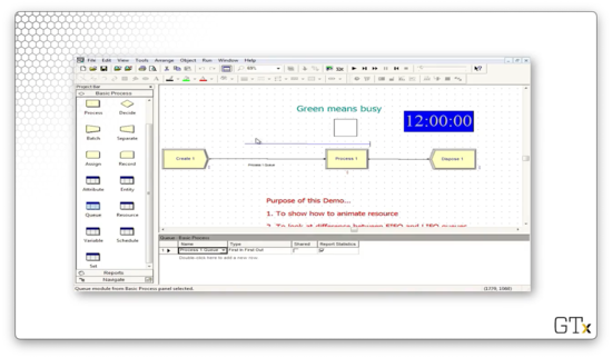
Notice that we have a green square above Process one, indicating that the server is busy. We can create this animation by clicking on the resource icon from the toolbar.
Clicking this icon pulls up a dialog box where we can select the appropriate graphics.
We can edit a queue by double-clicking on it, which brings up a dialog box.
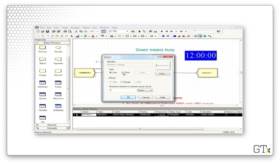
If we change the Type from "Line" to "Point", we can create a queue that looks like the following.
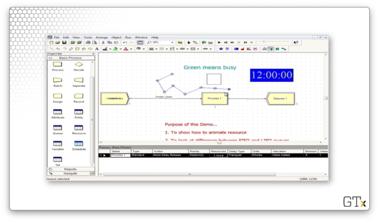
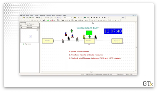
When we rerun the simulation, we see the customers line up according to the shape of the queue.
Let's edit the semantics of the queue now. If we click on the Queue spreadsheet, we see the queue - Process 1.Queue - in the bottom panel.
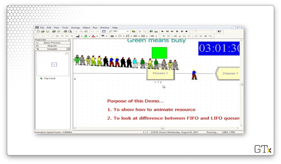
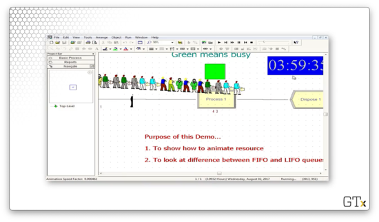
This queue has a Type of "First In First Out". We can click the Type dropdown and change this queue to "Last In First Out". Notice now how the first customer in the system stays at the end of the queue as other customers arrive.
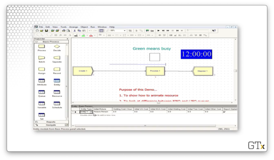
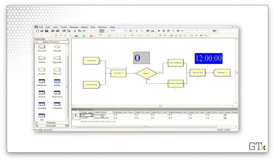
We can change what the customers look like by visiting the Entity spreadsheet. We can set the Initial Picture of the entity to "Picture.Person" to represent this entity as a person.
The Decide Module
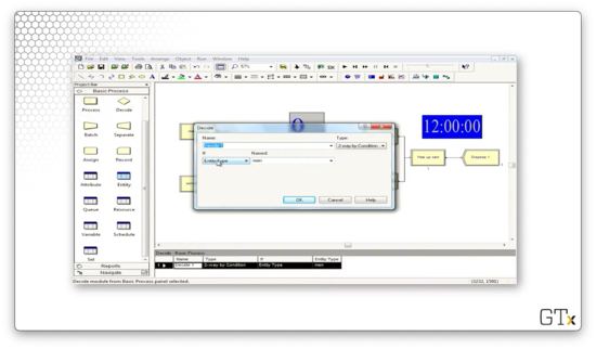
In this lesson, we will look at the Decide module. This module allows customers to make probabilistic and conditional decisions about what they are going to do next.
Decide Module
When an entity arrives at a Decide module, we can make one of the following decisions.
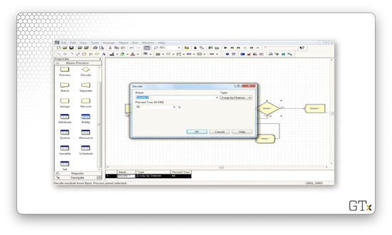
We can make a "2-way by Chance" decision, whereby we randomly send an entity to either of two locations. Correspondingly, we can make an "N-way by Chance" decision, where we send an entity to one of many locations based on specified probabilities. Note that in Arena, we express these probabilities as whole numbers, not decimals. For example, we represent 90% as 90, not 0.9.
Furthermore, there is a "2-way by Condition" choice, where we send an entity to one of two locations depending on whether a certain condition is satisfied. For example, we might send an entity to one store if it is raining and another if it is sunny. Symmetrically, the "N-way by Condition" choice sends the entity to any of N locations depending on a certain condition.
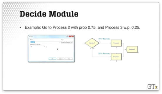
As an example, let's suppose we want to send an entity to Process 2 with a 75% probability and Process 3 with a 25% probability. We can specify this in the Decide dialog by selecting "2-way by Choice" from the Type dropdown and specifying 75 in the Percent True field.
DEMO
In this demo, we will look at a couple of examples involving the Decide module.
Let's look at the first example. Here we have a Create module, followed by an N-way by Condition Decide module, followed by three Dispose modules. Next to each Dispose module, we keep a tally of the proportion of customers that pass through that module.
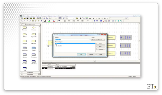
Let's look at the configuration for this Decide module. We see that this block has a Type of "N-way by Chance". We specified the percentages 30 and 50, and Arena is smart enough to know that there must be a third percentage of 20 so that the percentages sum to 100. So, the customer goes to the first Dispose block 30% of the time, the second Dispose block 50% percent of the time, and the final Dispose block 20% of the time.
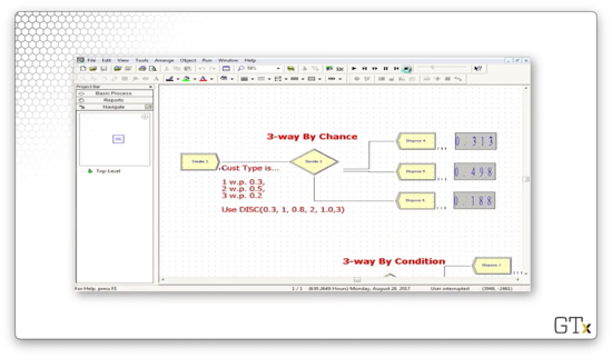
Let's run the simulation and see if we converge to those probabilities.
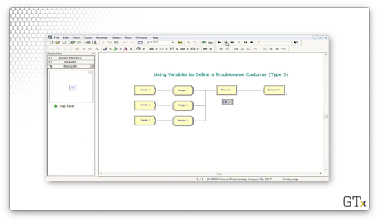
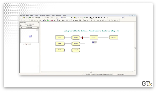
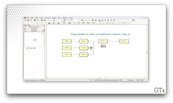
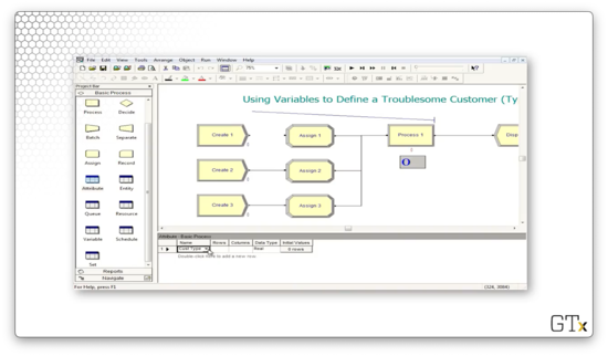
Now let's look at another example. Here we will look at a simulation involving the N-way by Condition Decide block.
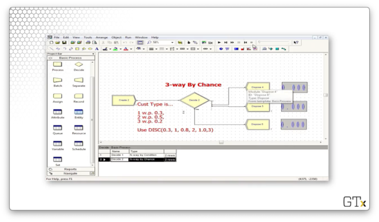
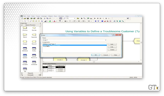
Notice that we are also using the Assign module. We use this module to assign variables and attributes to various components in our simulation. In this example, we assign a customer type to the entities that we generate in the Create module.
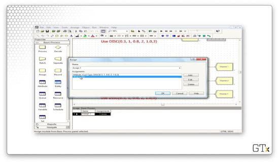
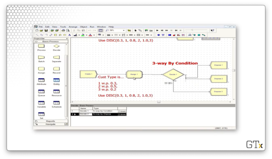
As we can see, we are assigning an attribute called "Cust Type" to the customer, where the value of the attribute is drawn from the "DISC(0.3, 1, 0.8, 2, 1.0, 3)" distribution. This distribution is discrete, whereby the value "1" appears 30% of the time, the value "2" appears 50% of the time, and the value "3" appears 20% of the time.
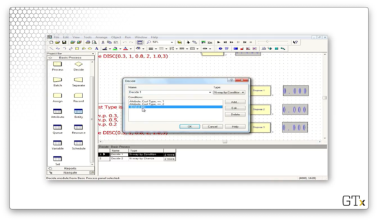
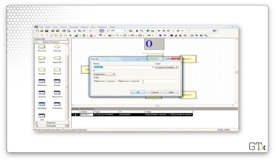
Now let's look at the Decide block configuration. Notice that the Type is "N-way by Condition", and the conditions are based on the customer type. The first condition is "Cust Type == 1", and the second condition is "Cust Type == 2". Again, Arena is smart enough to handle the final case for us.
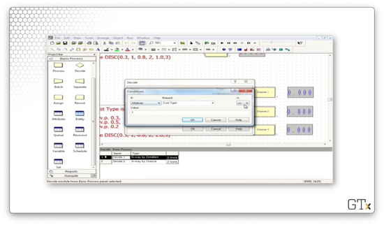
We can edit the condition by clicking the Edit button, which brings up the following dialog. We can see that we express the condition as an equality between the attribute "Cust Type" and the value "1".
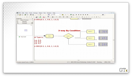
Let's run the simulation and see if the observed proportions converge to the expected values of 0.3, 0.5, and 0.2.
Let's look at one more demo. In this demo, we will generate arrivals of both men and women shoppers and then send them to different Process blocks based on their gender.
Let's look at the Decide block. Here we have a decision of type "2-way by Condition", where the condition checks if the entity type is equal to "men". If the entity is a man, we send them on the upper path; otherwise, we send them on the lower path.
We can specify the entity type in the Create block. For the Create block for the men, we see the Entity Type field is "men".
We can get the nice pictures for the men and women by going to the Entity spreadsheet and selecting "Picture.Man" for the entity of type "men" and "Picture.Woman" for the entity of type "women".
The Assign Module
In this lesson, we will look at the Assign module, which lets us give values to attributes and variables. Additionally, the Assign module allows us to assign graphics to entities.
Attributes
Each customer passing through the system has various properties or attributes unique to that customer. For example, we might have a customer named Tom who is six feet tall, weighs 160 pounds, loves baseball, and has an LDL cholesterol of 108. Tom has four different attributes - height, weight, hobby, cholesterol - which all have corresponding values.
We might have another customer, Justin B., who is four eleven, weighs 280 pounds, loves eating lard, and has an LDL cholesterol of 543. Both customers have the same four attributes, but the values of each attribute are different.
Attributes need to be numerical, so we may have to encode certain categorical attributes. For instance, we could associate the number 11 with baseball and the number 28 with eating lard.
Variables
Unlike attributes, whose values are specific to each customer, variables are global. If we change a variable anywhere in Arena, it gets changed everywhere. For example, we might maintain and global Work in Process (WIP) variable, which we increment any time an entity is created and decrement any time an entity is disposed.
Assign Module
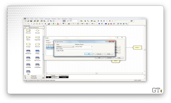
We use the Assign module to assign attributes, variables, and other values. In the following picture, we are changing an attribute called "Weight" to 160.
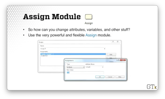
We can also use the Assign module to associate pictures with entities, such as the men and women we saw in a previous demo.
DEMO
In this demo, we will take a further look at the Assign module. Here's our model.
In the first Assign module, we assign a picture, Picture.Man, to the customers we generated in the Create module.
Next, we have a Process module, where the customers perform a Seize Delay Release on a barber that serves them in fifteen minutes on average.
After the Process module, we have a Decide block that involves a 2-way by Chance decision. In this block, 90% of the customers are satisfied and leave.
The remaining 10% of customers travel through another Assign block and then return to the Process module because they weren't satisfied with their first haircut.
Let's change the distribution of service times to an expression named "service time".
We can define "service time" in the Assign block. Specifically, we associate an attribute called "service time" with each entity we generate, which will subsequently be read by the Process block. Let's specify the service time as "tria(5,15,25)", a triangular distribution parameterized by a min, mode, and max of 5, 15, and 25.
If we run the simulation, we notice something funny - the picture for the dissatisfied customers changes from a man to a woman in the second Assign block.
Let's look at how we did that. We simply assigned the picture to a new value, Picture.Woman, in that Assign block.
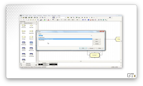
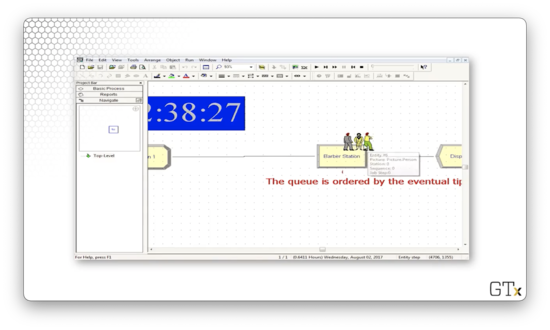
Let's look at another example. This time we will order the queue by the eventual tip that the customer will give.
Let's look at the Assign block. We have the Entity.Picture attribute set to Picture.Person, which randomly selects between a man and a woman. More interestingly, we have the "eventual_tip" attribute, which is drawn from a "NORM(10, 5)" distribution.
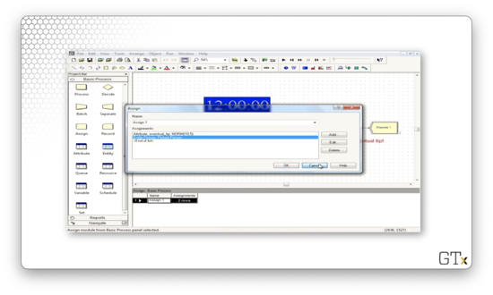
How can we specify the order for the queue? Let's go to the Queue spreadsheet and look at the Barber Station.Queue. Here we see the Type field set to "Highest Attribute Value" and the Attribute Name field set to "eventual_tip". This configuration means that we order the queue by the "eventual_tip" attribute on the entities.
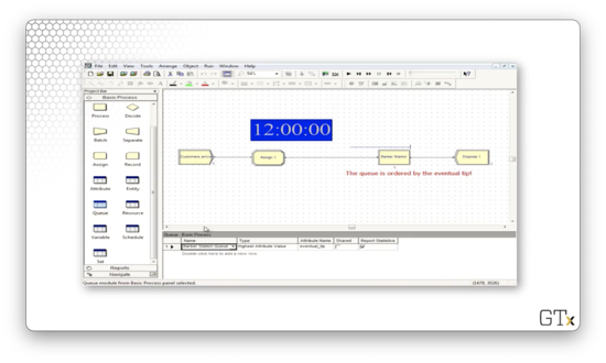
We can watch this scenario play out. Consider this queue setup.

Now consider the queue after another arrival.
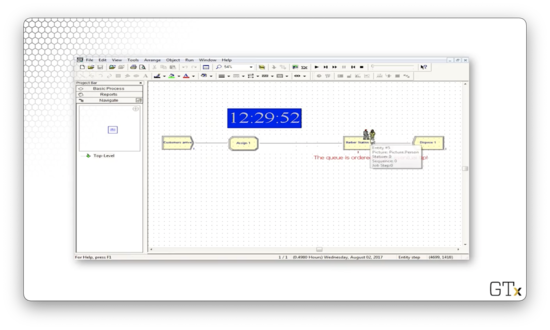
Notice how the customer who arrived later is before the other customer in the queue. Let's try again.
Again, the more recent customer goes to the front of the line because that customer offers the highest tip of the three in the queue.
Attribute, Variable, Entity Spreadsheets
In this lesson, we will look at the Attribute, Variable, and Entity spreadsheets.
Spreadsheets
The Attribute spreadsheet keeps track of existing attributes that you might define in an Assign module. Attributes can be real values or vectors. For example, we might have a three-element vectorized attribute called "height". The Variable spreadsheet looks pretty much the same, except that it controls variables instead of attributes.
The Entity spreadsheet allows us to set the initial picture for our customers, along with a few other properties. We will likely only use it to set customer pictures.
DEMO
In this demo, we will create three different types of entities and send them all through the same Process.
In the first Create-Assign component, we generate arrivals of women.
In the second Create-Assign component, we generate arrivals of men.
In the third Create-Assign component, we generate arrivals of entities that look like trucks.
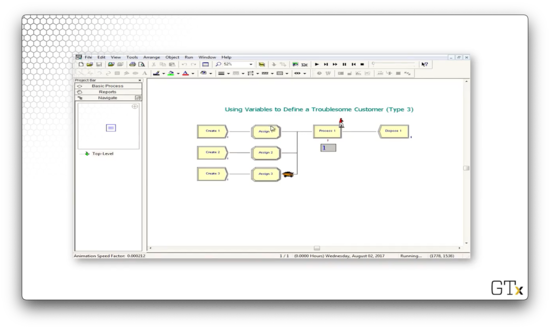
Let's step through the first few steps of this simulation. We generate three arrivals: a woman, a man, and a truck. The woman receives service first and exits the system. The man receives service next and also exits. The truck receives service next yet never seems to exit. By the time we stop the simulation, there are sixteen customers in the queue.
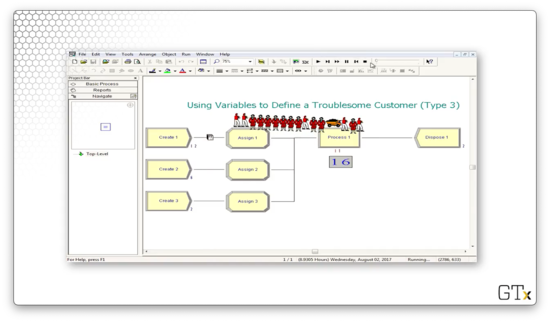
If we look at the configuration for the Process block, we see that the delay type is based on the expression "Expo(mean(Cust Type))".
We assign the "Cust Type" attribute in the Assign module. We assign a different value - "1", "2", or "3" - for each of the three types of arrivals we generate.
If we look at the Attribute spreadsheet, we can see the "Cust Type" attribute.
If we look at the Variable spreadsheet, we can see the "mean" variable that we have also defined. This variable is a vector with three elements, with indices starting at one: 0.5, 0.5, and 20.
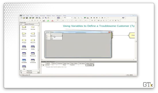
To retrieve the mean service time for a particular entity, we index into this vector with the entity's "Cust Type". With that in mind, we can see that women and men have a mean service time of 0.5 time units. On the other hand, trucks have a mean service time of 20 time units, which is forty times larger than the other two.
Arena Internal Variables
In this lesson, we will focus on Arena's internal variables, which automatically update and recalculate themselves as the simulation progresses. We can use these variables to make decisions based on the simulation's current state.
Internal Variables
Like we said, Arena keeps track of and continuously updates numerous pieces of state as the simulation runs.
The variable TNOW keeps track of the current simulated time. Every time something happens in the simulation, Arena updates TNOW.
Additionally, the variable NR keeps track of the number of resource servers currently working. For example, NR(Barber) refers to the number of barbers currently in service.
Similarly, the variable NQ keeps track of the number of customers in a particular queue. For example, NQ(Process 1.Queue) refers to the number of customers in line waiting for Process one.
Furthermore, the variable NumberOut refers to the number of customers that have left a particular module. For example, Create 1.NumberOut refers to the number of customers that have left a module named Create 1.
We can learn about many more internal variables by looking at the "Build Expression" menu.
DEMO
In this demo, we will look at how to make customers pick the shorter of two queues. Here's our setup.
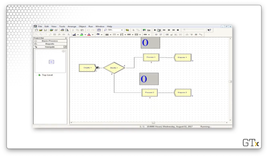
Let's look at the Decide block to get a sense of how this flow works. As we can see, we have a 2-way by Condition decision here, where we choose Process one if NQ(Process 1.Queue) < NQ(Process 2.Queue). In other words, if Process one's queue is shorter than Process two's, go to Process one. Otherwise, go to Process two.
Displaying Variables, Graphs, Results
In this lesson, we will discuss how we display the values of certain variables in real-time, construct useful graphs, and produce meaningful output files.
Getting Information
We might be curious as to how we display information as the simulation is running. Arena provides a toolbar with several different features. We can create a clock or calendar to keep track of time. We can maintain variable displays, which show the values of the variables in realtime. We can also generate histograms and graphs.
When the simulation ends, Arena automatically generates an output report that gives information and statistics on server usage, queue length, customer waits and cycle times, and other user-defined quantities.
DEMO
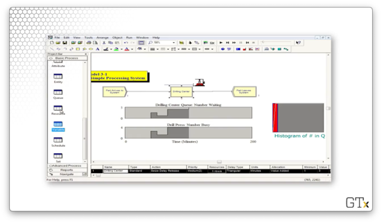
In this demo, we will look at a drill press simulation and talk about some of Arena's display and graphics capabilities.
As always, we have our Create-Process-Dispose setup, and we perform a Seize Delay Release of one resource in the Process block. Along the way, we will make a few graphs. One graph will show the number of people waiting in queue as a function of time, a second will show the number of drill press servers busy as a function of time, and a third will show a histogram of the number of people in the queue.
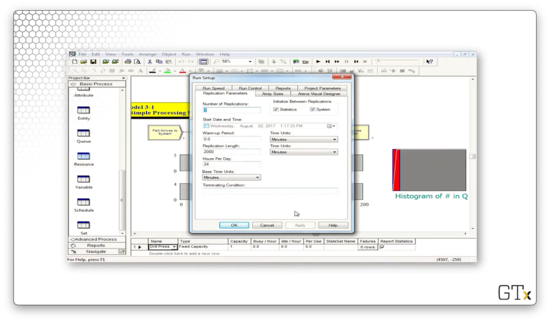
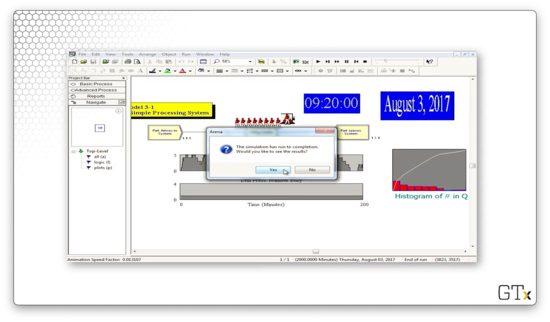
If we look at the Replication Parameters tab in the Run Setup dialog, which we access from the Run > Setup menu, we see that we will run this simulation for 2000 minutes.
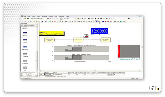
We will also add a digital clock to the workspace area so we can watch the time pass. Remember that we can add this feature by clicking on the Clock icon in the toolbar.
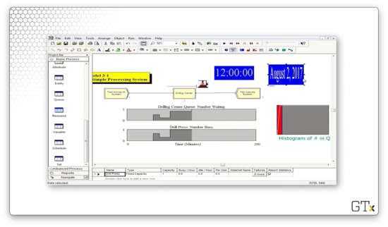
Furthermore, we will add a calendar. To do so, we click on the Calendar icon, right next to the Clock icon.
Let's take a look at the simulation.
Let's change the mean interarrival time from "4" to "3.4" to more closely match the mean service time, which is roughly 3.33 minutes.
Since we are making customers arrive more quickly, we expect lines to be longer.
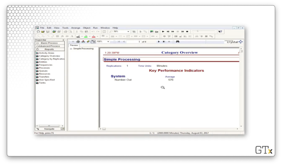
Once the simulation ends, we get a dialog asking us if we want to see the results. Let's click "Yes".
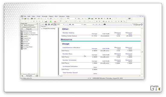
Here we have a four-page Crystal Report. This report gives us several key performance indicators. For example, we see here that "Number Out" is 576, which means that 576 customers have left our system after receiving service.
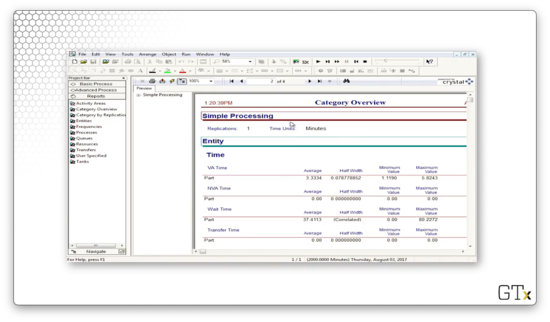
On page two, we can see the times spent in various parts of the system. For example, we see "Wait Time" has an average of "37.4", which means that customers waited for an average of 37.4 minutes in the queue.
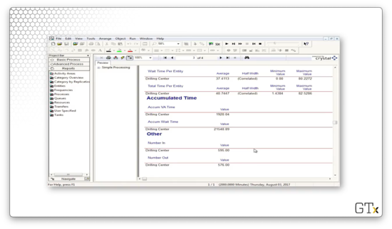
Page three gives us information about how much time entities spent in the drilling center. We can see that customers waited, on average, about 37 minutes and received service, on average, in about 3 minutes, for a total processing time of 40 minutes.
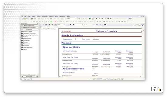
Furthermore, we can see that 595 customers entered and 576 left, which means that there were 19 customers still in the system when we ended the simulation.
On the fourth page, we see information about the drill process queue. For example, we can see the average waiting time in the queue and the average number of customers in the queue throughout the simulation.
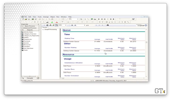
Finally, we can take a look at server usage information. For example, we can see that the server is busy 96% of the time. This observation makes sense since we generated customers almost as quickly as the server could process them.
Batch, Separate, Record Modules
In this lesson, we will discuss the Batch Separate and Record modules.
Batch Module
The Batch module combines ("batches") multiple customers into one super-customer.
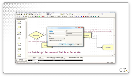
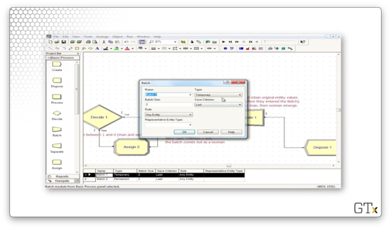
Let's look at how we can configure the Batch module. We can set the batch size by specifying a value in the "Batch Size" field. Here, we have entered "3", which means that we will accumulate three customers into one super-customer. Additionally, we have selected "Permanent" from the Type dropdown. We create a permanent batch when we don't need to retain information about the individual customers.
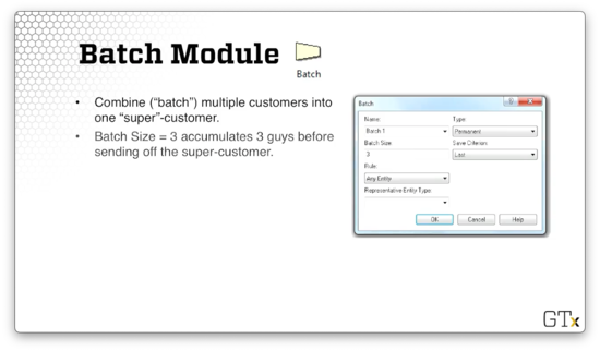
If we want to reconstitute the original customers eventually, we can select "Temporary" from the Type dropdown. Note that we need to split temporary batches to dispose of the constituent customers.
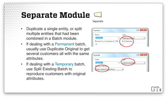
Separate Module
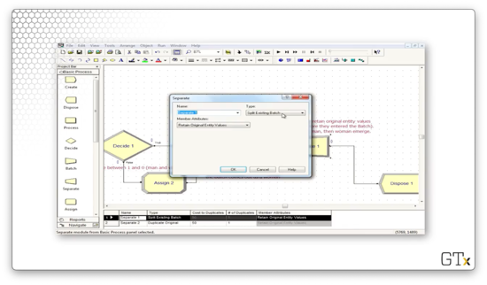
The Separate module can do two things: first, it can duplicate a single entity, and; second, it can split multiple entities that have been combined in a Batch module.
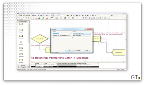
If we are dealing with a permanent batch, we usually will select "Duplicate Original" from the Type dropdown to get several clones of the super-customer.
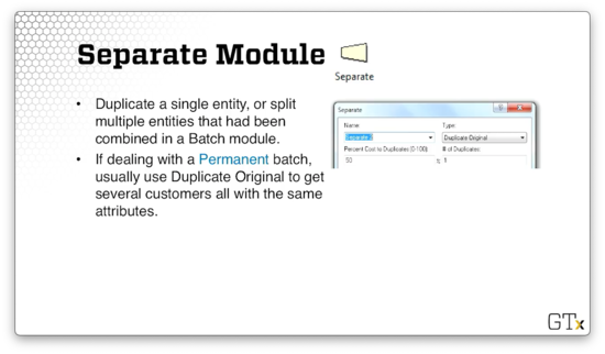
If we are dealing with a temporary batch, we can select "Split Existing Batch" from the Type dropdown to reproduce the original customers and their attributes.
Record Module
The Record module collects statistics when an entity passes through it. We will talk more about this module as we encounter it in future examples.
DEMO
In this demo, we will look at some features of the Batch, Separate, and Record modules.
Let's look at our first setup.
Here, we generate arrivals of women from a Create block. These arrivals pass through an Assign block and then a Decide block, where every other woman is sent to the bottom path and transformed into a man. Next, we hit the Batch module, where we accumulate two customers - a man and a woman - into one woman super-customer. Finally, in the Separate block, we duplicate the super-customer and dispose of them both.
Let's look at the configuration for the Batch block. Notice that we specify a batch size of two and a type of "Permanent". Why do we combine a man and a woman into a woman? We specify "Last" in the Save Criterion dropdown, and, since the woman arrives last, the batch looks like a woman.
Let's look at the Separate module now. Here we have selected "Duplicate Original" from the Type dropdown. We have also specified "1" in the # of Duplicates field, so we create one duplicate of the woman super-customer, sending two in total to the Dispose block.
Let's consider a second example. This time, everything is basically the same as the first example except that a man and a woman emerge from the Separate block.
Let's look at the Batch configuration. Here we have selected "Temporary" from the Type dropdown.
Let's look at the Separate block. We have selected "Split Existing Batch" from the Type dropdown, so we will break up our super-customer into its constituent entities.
Run, Setup, Control
In this lesson, we will look at several simple features that will ensure that our simulations execute efficiently.
Run Setup
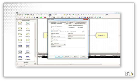
The Run > Setup menu gives us a lot of functionality. Often, we will look specifically at the Replication Parameter tab.
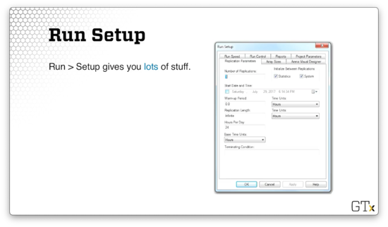
We can specify the number of times we run the simulation in the Number of Replications field. By default, the simulation runs once, but we often need to rerun simulations many times to generate useful statistics.
We can control whether we start fresh with system state and statistics collection between simulation runs using the Initialize Between Replications checkboxes.
Additionally, we can specify how long we want to run the simulation before keeping data and collecting statistics in the Warm-up Period field. If we are interested in a steady-state simulation, for example, it doesn't make sense to start collecting data right at the start.
We can control how long each run takes using the Replication Length field. We usually measure simulation length in units of time, so we might say that we want to run the simulation for 24 hours.
If we don't want to run the simulation for a certain amount of time, but, instead, until a particular event/state occurs, we can specify this data in the Terminating Condition field. For example, we could state that we want to end the simulation once the queue size hits 100 customers.
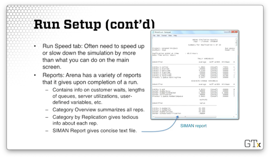
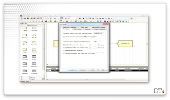
We can also adjust the speed of the simulation run with the Run Speed tab. Note that this tab offers much more control than the icons on the main screen.
We can look at the Reports tab to see and edit the collection of reports that Arena provides upon completing a simulation run. These reports contain information on customer wait times, queue lengths, server utilizations, user-defined variables, and more.
Furthermore, we can generate a "Category Overview" report that summarizes the individual replications. Alternatively, we can generate a "Category by Replication" report that provides tedious information about each replication. Finally, a "SIMAN" report provides a concise text file.
Run Control
From the Run > Setup dialog, we can click on the Run Control tab to see a variety of ways that we can run the simulation. For example, we can run the simulation in Batch mode, which turns off all graphics and results in extremely fast runs.
DEMO
In this demo, we will revisit our barber simulation. We have a Create-Process-Dispose setup, and each customer performs a Seize Delay Release of one barber.
Before we start, let's see how we can straighten these connections between modules. From the View menu, we can select Grid to create a grid in the main workspace area. Next, we select View > Snap to Grid to force all objects to align with the grid. From there, we can easily align our modules.
Let's look at some other parameters we can change about the simulation. We can head over to Run > Setup to get started. In the Run Speed tab, we can edit the Animation Speed Factor field to slow down or speed up the animation. Smaller numbers result in slower animations.
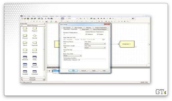
Now, let's check out the Replication Parameters tab. We can edit the Replication Length field to run the simulation for 100 hours instead of an infinite amount of time.
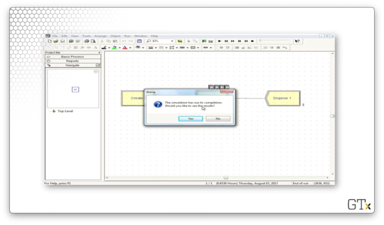
If we run the simulation to completion and check on the bottom of the Arena window, we see that we have run the simulation for 100.0000 hours.
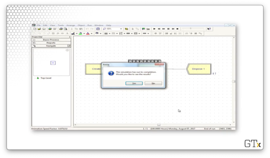
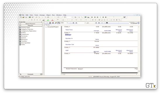
Let's look at the output, conveniently presented to us in SIMAN form as a .txt file.
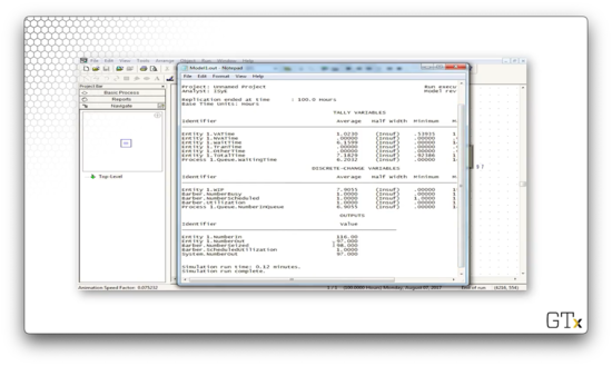
Here we can see that, for example, "Barber.Utilization" is 1.00, which means that the server was constantly working throughout the simulation. Additionally, we see "Entity 1.NumberIn" is 116 and "Entity 1.NumberOut" is 97. This observation indicates that 116 customers entered the simulation and 97 exited, which means that 19 customers were in the queue or service when the simulation ended.
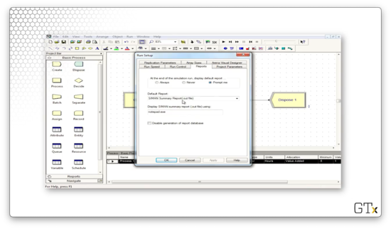
How do we generate this output? Back over in the Run > Setup dialog, we can select the Reports tab. Here we have selected the "SIMAN Summary Report" from the Default Report dropdown.
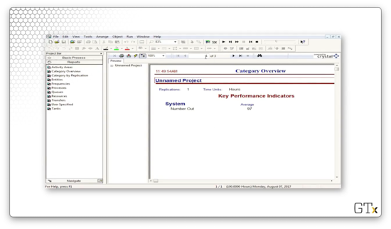
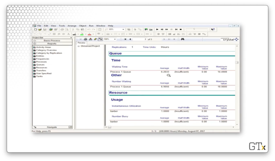
Let's change the default report to "Category Overview" and rerun the simulation. Here we have a three-page report. On page one, we see again that 97 customers left the system.
On page two, we can see that the work in process (WIP) variable was approximately eight, on average. This means that about eight customers were in line or service at any time during the simulation.
On page three, we can see information about the queue. For example, the average waiting time in the queue was 6.2 hours, and the average number of people waiting in the queue was 6.9. Additionally, we can see that server utilization was 100%.
Let's suppose that we hate the fact that we have a large queue. We can set a terminating condition in the Terminating Condition field in the Replication Parameters tab. If we want our simulation to terminate when the process queue has four customers, we can specify the terminating condition as NQ(Process 1.Queue) == 4.
If we rerun the simulation, we can see that the simulation ends once four people are in the queue.
OMSCS Notes is made with in NYC by Matt Schlenker.
Copyright © 2019-2023. All rights reserved.
privacy policy