Simulation
Generating Uniform Random Numbers
44 minute read
Notice a tyop typo? Please submit an issue or open a PR.
Generating Uniform Random Numbers
Introduction
Uniform(0,1) random numbers are the key to all random variate generation and simulation. As we have discussed previously, we transform uniforms to get other random variables - exponential, normal, and so on.
The goal is to produce an algorithm that can generate a sequence of pseudo-random numbers (PRNs) that "appear" to be i.i.d Uniform(0,1). Of course, these numbers are not truly uniform because they are neither independent of one another, nor are they random. However, they will appear random to humans, and they will have all the statistical properties of i.i.d Uniform(0,1) random numbers, so we are allowed to use them.
Such an algorithm has a few desired properties. As we said, we need to produce output that appears to be i.i.d Unif(0,1). We also need the algorithm to execute quickly because we might want to generate billions of PRNs. Moreover, we need the algorithm to be able to reproduce any sequence it generates. This property allows us to replicate experiments and simulation runs that rely on streams of random numbers.
In the next few lessons, we will look at different classes of Unif(0,1) generators. We'll start with some lousy generators, such as
- the output of a random device
- a table of random numbers
- the mid-square method
- the Fibonacci method
We will then move on to the more common methods used in practice: the linear congruential generators and the Tausworthe generator. Finally, we'll talk about hybrid models, which most people use today.
Some Lousy Generators
In this lesson, we will spend some time talking about poor generators. Obviously, we won't use these generators in practice, but we can study them briefly both for a historical perspective and to understand why they are so bad.
Random Devices
We'll start our discussion by looking at random devices. A coin toss is a random device that can help us generate values of zero or one randomly. Similarly, we can roll a die to generate a random number between one and six. More sophisticated random devices include Geiger counters and atomic clocks.
Naturally, random devices have strong randomness properties; however, we cannot reproduce their results easily. For example, suppose we ran an experiment based off of one billion die rolls. We'd have to store the results of those rolls somewhere if we ever wanted to replicate the experiment. This storage requirement makes random devices unwieldy in practice.
Random Number Tables
We can also use random number tables. These tables are relatively ubiquitous, although they have fallen out of use since the 1950s. This table, published by the RAND corporation, contains one million random digits and one hundred thousand normal random variates. Basically, folks used a random device to generate random numbers, and then they wrote them down in a book.
How do we use this book? Well, we can simply flip to a random page, put our finger down in the middle of the page, and start reading off the digits.
While this approach has strong reproducibility and randomness properties, it hasn't scaled to meet today's needs. More specifically, a finite sequence of one million random numbers is just not sufficient for most applications. We can consume a billion random numbers in seconds on modern hardware. Additionally, once the digits were tabled, they were no longer random.
Mid-Square Method
The mid-square method was created by the famous mathematician John von Neumann. The main idea here is we take an integer, square it, and then use the middle part of that integer as our next random integer, repeating the process as many times as we need. To generate the Uniform(0,1) random variable, we would divide each generated integer by the appropriate power of ten.
Let's look at an example. Suppose we have the seed . If we square , we get , and we set equal to the middle four digits: . We can generate in a similar fashion: , so . Now, since we are taking the middle four integers, we generate the corresponding Uniform(0,1) random variate, , by dividing by . For example, , and by similar arithmetic.
Unfortunately, it turns out that there is a positive serial correlation in the 's. For example, a very small often follows a very small , more so than we would expect by random chance. More tragically, the sequence occasionally degenerates. For example, if , then the sequence ends up producing only zeros after a certain point.
Fibonacci and Additive Congruential Generators
The Fibonacci and additive congruential generators, not to be confused with the linear congruential generators, are also no good.
Here is the expression for the Fibonacci generator, which got its name got its name from the famed sequence that involves adding the previous two numbers to get the current number.
For this sequence, and are seeds, and is the modulus. Remember that if and only if is the remainder of . For example, .
Like the mid-square method, this generator has a problem where small numbers frequently follow small numbers. Worse, it turns out the one-third of the values for each subsequent uniform are impossible to calculate. Particularly, it is impossible to compute an , such that , or . Those two configurations should occur one-third of the time, which means that this generator does not have strong randomness properties.
Linear Congruential Generator
In this lesson, we will ditch the lousy pseudo-random number generators and turn to a much better alternative: the linear congruential generator (LCG). Variations of LCGs are the most commonly used generators today in practice.
LCGs
Here is the general form for an LCG. Given a modulus, , and the constants and , we generate a pseudo-random integer, , and its corresponding Uniform(0,1) counterpart, , using the following equations:
We choose , , and carefully to ensure both that the 's appear to be i.i.d uniforms and that the generator has long periods or cycle lengths: the amount of time until the LCG starts to repeat.
Multiplicative generators are LCGs where .
Trivial Example
Let's look at an example. Consider the following LCG:
Starting with the seed, , we can generate the following sequence of values:
Notice that this sequence starts repeating with after eight observations: . This generator is a full-period generator since it has a cycle length equal to . Generally speaking, we prefer full-period generators, but we would never use this particular generator in practice because the modulus is much too small.
Let's consider the following plot of all coordinate pairs. For example, the point corresponds to . Notice that we also include the point . We can observe that .
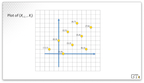
What's interesting about this plot is that the pseudo-random numbers appear to fall on lines. This feature is a general property of the linear congruential generators.
Easy Exercise
Consider the following generator:
Does this generator achieve full cycle? Let's find out:
If we seed this sequence with an odd number, we only see odd numbers. Similarly, if we seed this sequence with an even number, we only see even numbers. Regardless, this sequence repeats after four observations, and, since the modulus is eight, this generator does not achieve full cycle.
Better Example
Let's look at a much better generator, which we have seen before:
This particular generator has a full-period (greater than two billion) cycle length, except when .
Let's look at the algorithm for generating each and :
As an example, if , then:
What Can Go Wrong?
As we saw, we can have generators like , which only produce even integers and are therefore not full-period. Alternatively, the generator is full-period, but it produces very non-random output: , , and so on.
In any case, if the modulus is "small", we'll get unusably short cycling whether or not the generator is full period. By small, we mean anything less than two billion or so. However, just because is big, we still have to be careful because subtle problems can arise.
RANDU Generator
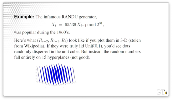
Let's take a look at the RANDU generator, which was popular during the 1960s:
Unfortunately, the numbers that this LCG generates are provably not i.i.d., even from a statistical point of view.
Let's take a sufficiently large and plot the points within a unit cube. If the numbers generated from this sequence were truly random, we would see a random dispersion of dots within the cube. However, the random numbers fall entirely on fifteen hyperplanes.
Exercises
Tausworthe Generators
In this lesson, we will look at the Tausworthe generator.
Tausworthe Generator
Let's take a look at the Tausworthe generator. We will define a sequence of binary digits, as:
In other words, we calculate each by taking the sum of the previous products, where . We take the entire sum , so every is either a one or a zero.
Instead of using the previous entries in the sequence to compute , we can use a shortcut that saves a lot of computational effort, which takes the same amount of time regardless of the size of :
Remember that any can only be either or . Consider the following table:
Now, let's consider the operator. If we think of the operator as, colloquially, "either this or that", we can think of the as "either this or that, but not both"; indeed, is an abbreviation of "eXclusive OR". Let's look at the truth table:
Thus, we can see that and are indeed equivalent. Of course, we might use an even simpler expression to compute , which doesn't involve :
To initialize the sequence, we need to specify, .
Example
Let's look at an example. Consider . Thus, for , . For example, and . Let's look at the first 36 values in the sequence:
Generally, the period of these bit sequences is . In our case, , so . Indeed, the thirty-second bit restarts the sequence of five ones that we see starting from the first bit.
Generating Uniforms
How do we get Unif(0,1) random variables from the 's? We can take a sequence of bits and divide them by to compute a real number between zero and one.
For example, suppose . Given the sequence of bits in the previous sequence, we get the following sequence of randoms:
Tausworthe generators have a lot of potential. They have many nice properties, including long periods and fast calculations. Like with the LCGs, we have to make sure to choose our parameters - , , , and - with care.
Generalizations of LCGs
In this lesson, we will return to the LCGs and look at several generalizations, some of which have remarkable properties.
A Simple Generalization
Let's consider the following generalization:
Generators of this form can have extremely large periods - up to if we choose the parameters correctly. However, we need to be careful. The Fibonacci generator, which we saw earlier, is a special case of this generalization, and it's a terrible generator, as we demonstrated previously.
Combinations of Generators
We can combine two generators, and , to construct a third generator, . We might use one of the following techniques to construct the 's:
- Set equal to
- Shuffling the 's and 's
- Set conditionally equal to or
However, the properties for these composite generators are challenging to prove, and we should not use these simple tricks to combine generators.
A Really Good Combined Generator
The following is a very strong combined generator. First, we initialize . Next, for :
As crazy as this generator looks, it only requires simple mathematical operations. It works well, it's easy to implement, and it has an amazing cycle length of about .
Some Remarks
Matsumoto and Nishimura have developed the "Mersenne Twister" generator, which has a period of . This period is beyond sufficient for any modern application; we will often need several billion PRNs, but never more than even . All standard packages - Excel, Python, Arena, etc. - use one of these "good" generators.
Choosing a Good Generator - Theory
In this lesson, we will discuss some PRN generator properties from a theoretical perspective, and we'll look at an amalgamation of typical results to aid our discussion.
Theorem
Suppose we have the following multiplicative generator:
This generator can have a cycle length of at most , which means that this generator is not full-cycle. To make matters worse, we can only achieve this maximum cycle length when is odd and or , for some .
For example, suppose . Note that and . Consider the following sequence of values:
We can see that we have cycled after entries. What happens to the cycle length if is even?
Here, we cycle after entries. Let's look at the cycle for . As we can see, our cycle length increases back to :
Finally, let's look at the sequence when . As we can see, when we seed the generator with this value, our cycle length drops to four.
Theorem
Suppose we have the following linear congruential generator:
This generator has full cycle if the following three conditions hold:
- and are relatively prime
- is a multiple of every prime which divides
- is a multiple of if divides
Let's look at a corollary to this theorem. Consider the following special case of the general LCG above:
This generator has full cycle if is odd and for some .
Theorem
Suppose we have the following multiplicative generator:
This generator has full period (, in this case), if and only if the following two conditions hold:
- divides
- for all integers , does not divide
We define the full period as in this case because, if we start at , we just cycle at zero.
For , it can be shown that multipliers yield full period. In some sense, is the "best" multiplier, according to this paper by Fishman and Moore from 1986.
Geometric Considerations
Let's look at consecutive PRNs, , generated from a multiplicative generator. As it turns out, these -tuples lie on parallel hyperplanes in a -dimensional unit cube.
We might be interested in the following geometric optimizations:
- maximizing the minimum number of hyperplanes in all directions
- minimizing the maximum distance between parallel hyperplanes
- maximizing the minimum Euclidean distance between adjacent -tuples
Remember that the RANDU generator is particularly bad because the PRNs it generates only lie on 15 hyperplanes.
One-Step Serial Correlation
We can also look at a property called one-step serial correlation, which measures how adjacent are correlated with each other. Here's a result from this paper by Greenberg from 1961:
Remember that is the multiplicative constant, is the additive constant, and is the modulus.
This upper bound is very small when is in the range of two billion, and is, say, . This result is good because it demonstrates that small 's don't necessarily follow small 's, and large 's don't necessarily follow large 's.
Choosing a Good Generator - Stats Test
In this lesson, we'll give an overview of various statistical tests for goodness-of-fit and independence. We'll conduct specific tests in subsequent lessons.
Statistical Tests Intro
We will look at two general classes of tests because we have a couple of goals we want to accomplish when examining how well pseudo-random number generators perform.
We run goodness-of-fit tests to ensure that the PRNs are approximately Unif(0,1). Generally speaking, we will look at the chi-squared test to measure goodness-of-fit, though there are other tests available. We also run independence tests to determine whether the PRNs are approximately independent. If a generator passes both tests, we can assume that it generates approximately i.i.d Unif(0,1) random variables.
All the tests that we will look at are hypothesis tests: we will test our null hypothesis () against an alternative hypothesis ().
We regard as the status quo - "that which we currently believe to be true". In this case, refers to the belief that the numbers we are currently generating are, in fact, i.i.d Unif(0,1).
If we get substantial, observational evidence that is wrong, then we will reject it in favor of . In other words, we are innocent until proven guilty, at least from a statistical point of view.
When we design a hypothesis test, we need to set the level of significance, , which is the probability that we reject , given it is true: . Typically, we set equal to or . Rejecting a true is known as a Type I Error.
Selecting a value for informs us of the number of observations we need to take to achieve the conditional probability to which refers. For example, if we set to a very small number, we typically have to draw more observations than if we were more flexible with .
We can also specify the probability of a Type II Error, which is the probability, , of accepting , given that it is false: . We won't focus on much in these lessons.
Usually, we are much more concerned with avoiding incorrect rejections of , so tends to be the more important of the two measures.
For instance, suppose we have a new anti-cancer drug, and it's competing against our current anti-cancer drug, which has average performance. Our null hypothesis would likely be that the current drug is better than the new drug because we want to keep the status quo. It's a big problem if we reject this hypothesis and replace it with a less effective drug; indeed, it's a much worse situation than not replacing it with a superior drug.
Choosing a Good Generator - Goodness-of-Fit Tests
In this lesson, we'll look at the chi-squared goodness-of-fit test to check whether or not the PRNs we generate are indeed Unif(0,1). There are many goodness-of-fit tests in the wild, such as the Kolmogorov-Smirnov test and the Anderson-Darling test, but chi-squared is the most tried-and-true. We'll look at how to do goodness-of-fit tests for other distributions later.
Chi-Squared Goodness-of-Fit Test
The first thing we need to consider when designing this test is what our null hypothesis ought to be. In this case, we assume that our PRNs are Unif(0,1). Formally, : . As with all hypothesis tests, we assume that is true until we have ample evidence to the contrary, at which point we reject .
To start, let's divide the unit interval, , into adjacent sub-intervals of equal width: . If our alleged uniforms are truly uniform, then the probability that any one observation will fall in a particular sub-interval is .
Next, we'll draw observations, , and observe how many fall into each of the cells. Let equal the number of 's that fall in sub-interval . Given trials, and a probability of of landing in sub-interval , we see that each is distributed as a binomial random variable: . Note that we can only describe in this way if we assume that the 's are i.i.d.
Since is a binomial random variable, we can define the expected number of 's that will fall in cell as: . Remember that, by definition, the expected value of a Bin() random variable is .
We reject the null hypothesis that the PRNs are uniform if the 's don't match the 's well. In other words, if our observations don't match our expectations, under the assumption that is true, then something is wrong. The only thing that could be wrong is the null hypothesis.
The goodness-of-fit statistic, , gives us some insight into how well our observations match our expectations. Here's how we compute :
Note the subscript of . All this means is that is a statistic that we collect by observation.
In layman's terms, we take the sum of the squared differences of each of our observations and expectations, and we standardize each squared difference by the expectation. Note that we square the difference so that negative and positive deviations don't cancel.
If the observations don't match the expectations, then will be a large number, which indicates a bad fit. When we talk about "bad fit" here, what we are saying is that describing the sequence of PRNs as being approximately Unif(0,1) is inappropriate: the claim doesn't fit the data.
As we said, is a binomial random variable. For large values of and , binomial random variables are approximately normal. If is the expected value of , then .
As it turns out, the quantity is a random variable, and, by dividing it by , we standardize it to a random variable with one degree of freedom. If we add up random variables, we get a random variable with degrees of freedom.
Note that the 's are correlated with one another; in other words, if falls in one sub-interval, it cannot fall in another sub-interval. The number of observations that land in one sub-interval is obviously dependent on the number that land in the other sub-intervals.
All this to say: we don't actually get degrees of freedom, in our resulting random variable, we only get . We have to pay a penalty of one degree of freedom for the correlation. In summary, by the central limit theorem, , if is true.
Now, we can look up various quantiles for distributions with varying degrees of freedom, , where we define a quantile, as: . In our case, we reject the null hypothesis if our test statistic, , is larger than , and we fail to reject if .
The usual recommendation from an introductory statistics class for the goodness-of-fit test is to pick large values for and : should be at least five, and should be at least 30.
However, when we test PRN generators, we usually have massive values for both and . When is so large we can't find tables with values for , we can approximate the quantile using the following expression:
Note that is the appropriate standard normal quantile.
Illustrative Example
Suppose we draw observations, and we've divided the unit interval into equal sub-intervals. The expected number of observations that fall into each interval is . Let's look at the observations we gathered:
Let's compute the goodness-of-fit statistic:
Since , we are looking at a distribution with four degrees of freedom. Let's choose . Now, we need to look up the quantile in a table, which has a value of 9.49. Since our test statistic is less than the quantile, we fail to reject . We can assume that these observations are approximately uniform.
Choosing a Good Generator - Independence Tests I
In this lesson, we'll look at the so-called "runs" tests for independence of PRNs. There are many other tests - correlation tests, gap test, poker tests, birthday tests, etc. - but we'll focus specifically on two types of runs tests.
Interestingly, we find ourselves in something of a catch-22: the independence tests all assume that the PRNs are Unif(0,1), while the goodness-of-fit tests all assume that the PRNs are independent.
Independence - Runs Tests
Let's consider three different sequences of coin tosses:
In example A, we have a high negative correlation between the coin tosses since tails always follows heads and vice versa. In example B, we have a high positive correlation, since similar outcomes tend to follow one another. We can't see a discernible pattern among the coin tosses in example C, so observations might be independent in this sequence.
A run is a series of similar observations. In example A above, there are ten runs: "H", "T", "H", "T", "H", "T", "H", "T", "H", "T". In example B, there are two runs: "HHHHH", "TTTTT". Finally, in example C, there are six runs: "HHH", "TT", "H", "TT", "H", "T".
In independence testing, our null hypothesis is that the PRNs are independent. A runs test rejects the null hypothesis if there are "too many" or "too few" runs, provided we quantify the terms "too many" and "too few". There are several types of runs tests, and we'll look at two of them.
Runs Test "Up and Down"
Consider the following PRNs:
In the "up and down" runs test, we look to see whether we go "up" or "down" as we move from PRN to PRN. Going from to , we go up. Going from to , we go up. Going from to , we go down. From to , we go down again.
Let's transform our sequence of PRNs into one of plusses and minuses, where a plus sign indicates going up, and a minus sign indicates going down:
Here are the associated runs - there are six in total - demarcated by commas:
Let denote the total number of up and down runs out of the observations. Like we said, in this example. If is large (say, ), and the 's are indeed independent, then is approximately normal, with the following parameters:
Let's transform into a standard normal random variable, , which we accomplish with the following manipulation:
Now we can finally quantify "too large" and "too small". Specifically, we reject if the absolute value of is greater than the standard normal quantile:
Up and Down Example
Suppose we have observed runs over observations. Given these variables, is approximately normal with the following parameters:
Let's compute :
If , then and we reject , thereby rejecting independence.
Runs Test "Above and Below the Mean"
Let's look at the same sequence of PRNs:
Let's transform our sequence of PRNs into one of plusses and minuses, where a plus sign indicates that , and a minus sign indicates that :
Here are the associated runs - there are three in total - demarcated by commas:
If is large (say, ), and the 's are indeed independent, then the number of runs, , is again approximately normal, with the following parameters:
Note that refers to the number of observations greater than or equal to the mean and .
Let's transform into a standard normal random variable, , which we accomplish with the following manipulation:
Again, we reject if the absolute value of is greater than the standard normal quantile:
Above and Below the Mean Example
Consider the following sequence of observations:
In this case, we have observations above the mean and observations below the mean, as well as runs. Without walking through the algebra, we can compute that .
Let's compute :
If , then , and we fail to reject . Therefore, we can treat the observations in this sequence as being independent.
Choosing a Good Generator - Independence Tests II (OPTIONAL)
In this lesson, we'll look at another class of tests, autocorrelation tests, that we can use to evaluate whether pseudo-random numbers are independent.
Correlation Test
Given a sequence of PRNs, , and assuming that each is Unif(0,1), we can conduct a correlation test against the null hypothesis that the 's are indeed independent.
We define the lag-1 correlation of the 's by . In other words, the lag-1 correlation measures the correlation between one PRN and its immediate successor. Ideally, if the PRNs are uncorrelated, should be zero.
A good estimator for is given by:
In particular, if is large, and is true:
Let's transform into a standard normal random variable, , which we accomplish with the following manipulation:
We reject if the absolute value of is greater than the standard normal quantile:
Example
Consider the following PRNs:
After some algebra, we get and . Notice how high our correlation estimator is; we might expect a robust rejection of the null hypothesis.
Let's compute :
If , then , and we fail to reject . Therefore, we can treat the observations in this sequence as being independent. In this case, observations is quite small, and we might indeed reject , given such a high correlation, if we were to collect more observations.
OMSCS Notes is made with in NYC by Matt Schlenker.
Copyright © 2019-2023. All rights reserved.
privacy policy