Simulation
Arena, Continued
43 minute read
Notice a tyop typo? Please submit an issue or open a PR.
Arena, Continued
Simple Two-Channel Manufacturing Example
In this lesson, we will put together everything we've learned and demo a two-channel manufacturing system. We are going to pay particular attention in this demo to our use of attributes.
In this example, we have two different types of arrival streams. We have type A parts, which show up one-at-a-time, and type B parts, which show up four-at-a-time. Type A parts show up slightly more often than type B parts. Type A parts feed into a Prep A server, and Type B parts feed into a Prep B server. Each prep server has different service times.
Both types of parts get processed by the same Sealer server. Interestingly, the Sealer has unique service time distributions for each of the two parts. As a result, the Sealer has to identify which part it is currently processing.
Finally, all parts undergo an inspection. If they pass inspection, they exit the system. Otherwise, they go to a Rework server, followed by another inspection. This time, regardless of whether they pass, they exit the system.
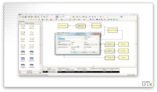
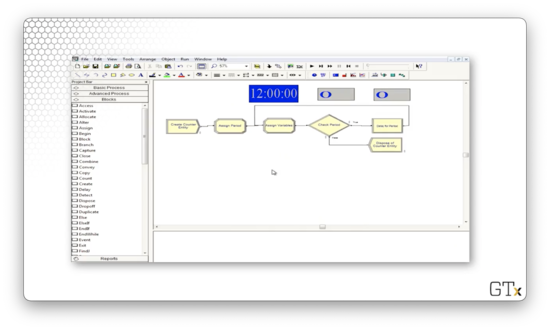
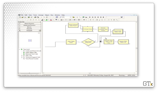
Let's look at a flowchart representing this model.
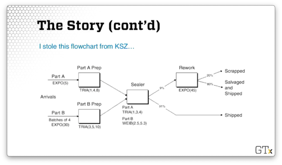
We generate Part A from an exponential distribution with a mean of five minutes. We generate Part B in batches of four from an exponential distribution with a mean of thirty minutes. Part A goes to a Prep server with service times generated from a triangular(1,4,8) distribution, while Part B goes to Prep server with service times generated from a triangular(3,5,10) distribution.
Both parts then head to the Sealer server, and Part A receives service according to a triangular(1,3,4) distribution, while Part B receives service according to a Weibull(2.5,5.3) distribution.
In any event, 91% of all parts coming out of the Sealer can be shipped immediately. The other 9% need to be reworked and head over to the Rework server. This server generates service times from an exponential distribution with a mean service time of 45 minutes. Of those reworked pieces, 20% are scrapped, and 80% are salvaged and shipped.
How do we handle different service times for Part A and Part B at the Sealer? We can pre-assign the service times as an attribute called Sealer Time in an Assign module immediately after each customer arrives. Then, the Sealer module can read the Sealer Time attribute and generate the appropriate service time.
Is there another way to model the processing time at the Sealer without having to assign a Sealer Time attribute ahead of time? Note that the entity types - Part A and Part B - are assigned automatically in the respective Create modules. We can leverage the entity type directly in the Sealer module; specifically, we can use a logical expression that checks against the entity type and returns the correct distribution.
Here is what that expression looks like: ((Entity.Type == Part A) * TRIA(1,3,4)) + ((Entity.Type == Part B) * WEIB(2.5,5.3)). Since the expression X == Y equals one if it is true and zero if it is false, we are essentially zeroing out the effect of the distribution of the complementary part when a part arrives. For example, if Entity.Type == Part A then the expression above reduces to 1 * TRIA(1,3,4) + 0, which equals TRIA(1,3,4).
We can also use the Assign module to store each customer's arrival time as an attribute (Arrival Time). We can use the Arena internal variable TNOW to retrieve the current time.
We can also record departure times just before parts get disposed. The difference between the arrival time and the departure time is the cycle time. We can calculate the average cycle times for any of the three categories of parts - those that pass on the first try, the second try, or those that fail on both.
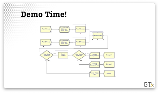
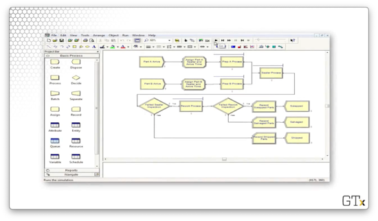
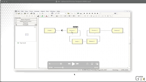
Here is what this model looks like in Arena.
DEMO
In this demo, we will walk through the two-channel manufacturing system we just described. Here's our setup.
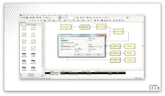
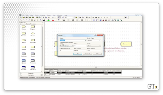
Notice that we have two different products, each with their own arrivals. Part A arrivals are generated from an EXPO(5) distribution, and the parts show up one at a time. Note as well that the Entity Type for these parts is "Part A".
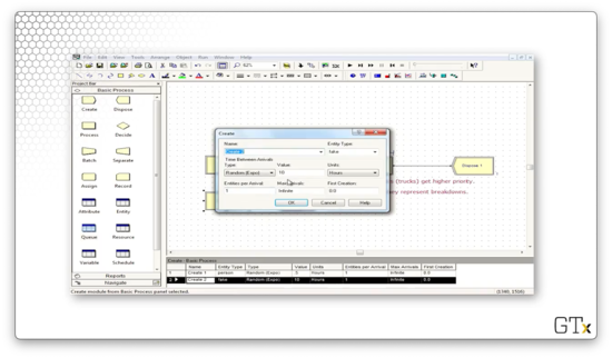
The arrivals for part B, on the other hand, are generated from an EXPO(30) distribution, and these parts show up four at a time. Correspondingly, the Entity Type for these parts is "Part B".
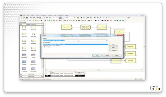
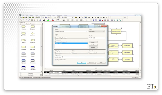
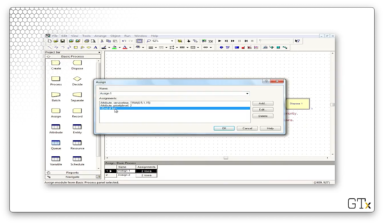
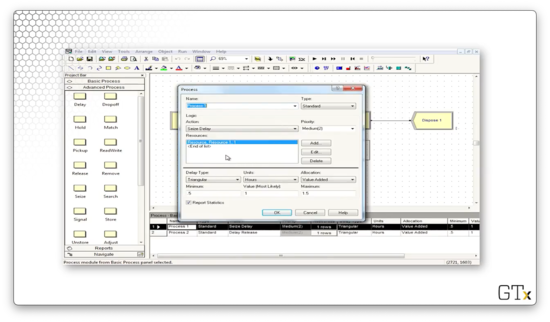
After the parts arrive, they immediately pass through an Assign block. Below is the configuration for the Assign block for part A. Here, we set two attributes: 'Sealer Time', which takes a value of TRIA(1,3,4), and 'Arrival Time', which takes a value of TNOW.
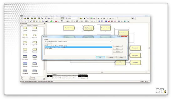
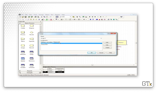
We again set the 'Arrival Time' attribute to TNOW for part B, but we set the 'Sealer Time' attribute to WEIB(2.5,5.3).
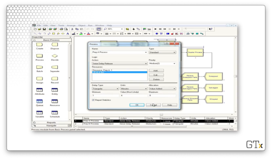
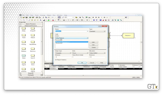
Both parts then head to their corresponding prep process. The prep processes for both parts perform a Seize-Delay-Release with service times from a TRIA(1,4,8) distribution.
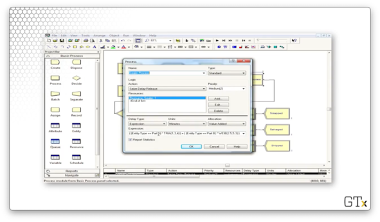
Now, let's look at the Sealer Process. We also perform a Seize-Delay-Release in this process, but the delay comes from the expression 'sealer time'. This expression reads an attribute of the same name off of the part, which refers to the appropriate distribution.
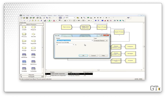
Next, we undergo the inspection to see if the processed part passes or fails inspection. Here is the configuration for the Decide block, which performs a "2-way by Chance" decision that is true - the part fails inspection - 9% of the time.
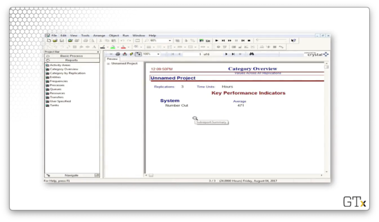
Let's run the entire simulation and generate some reports. As we can see from the first page of the report, we ran three replications, over which an average of 471 parts left our system.
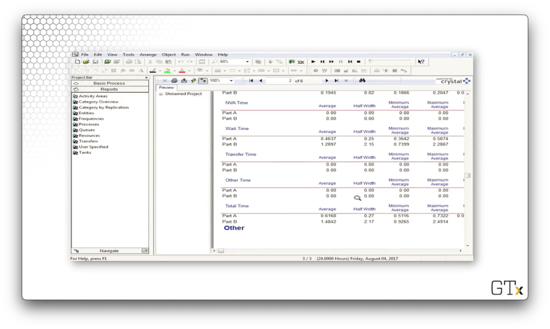
On page two, we can see information about wait times for both parts. On average, part A units had to wait 0.4637 hours, whereas part B units had to wait 1.2897 hours.
As a final note, we don't need to assign the sealer time as an attribute. We can replicate the exact same logic by reading off the Entity.Type attribute, which we set in the Create block.
Fake Customers
In this lesson, we'll talk about "fake" customers. The idea here is that these customers aren't real customers, and their purpose is just to do some specialized tasks that Arena might need in certain circumstances.
Fake Customers
We can use fake customers to accomplish various tasks in a simulation. As we said, these customers aren't real in the sense that we care about their waiting times or how they use resources. They can use resources, but only for certain reasons, and we don't care if they have to wait.
In this demo, we will use fake customers to calculate normal probabilities. In the call center example, we will use fake customers to track which time-period we're in. Furthermore, we can use fake customers as a breakdown demon; that is, we will use fake customers to trigger breakdowns.
DEMO
In this demo, we will calculate normal probabilities, based on successes and failures of certain observations, with a little help from fake customers. Specifically, we want to calculate the probability that a Norm(3,1) random variable is negative. Here's our setup.

First, we will generate one million customer arrivals, one hour at a time, using a Create block.
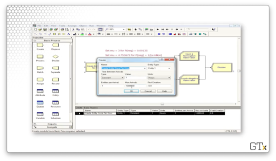
Next, we will use an Assign block to assign an attribute called "Normal Observation" - a Norm(3,1) random variable - to each customer.
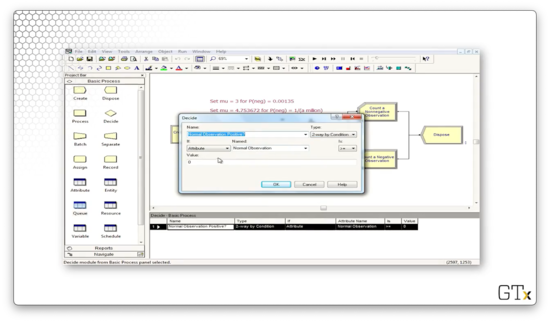
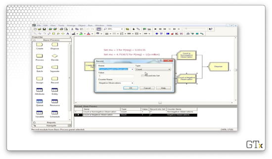
Next, we need to determine whether the attribute is negative or positive, so we need a Decide block. Notice that we have specified a decision of Type "2-way by Condition". This condition checks If an "Attribute" Named "Normal Observation" Is ">=" to the Value "0", which of course, is the conditional logic we just described in plain English.
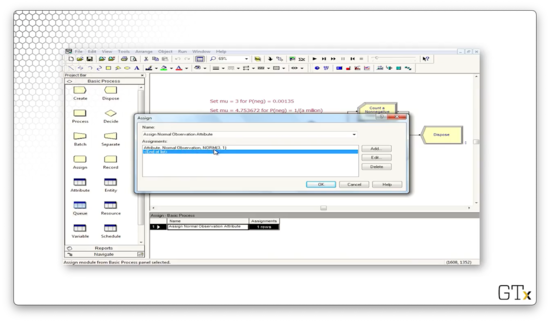
If the random variable is greater than zero, we record a nonnegative observation. Otherwise, we record a negative observation. Let's look at the Record block for the negative observation. Here, we select a Type of "Count" and a Value of "1", and we apply it to the counter named "Negative Observations".
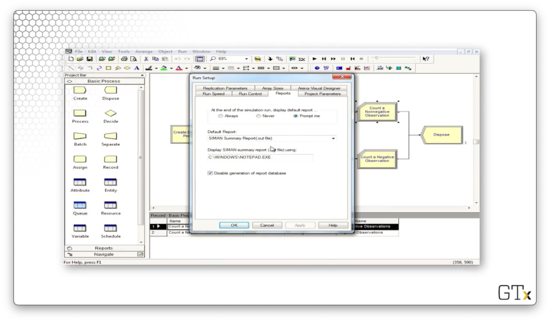
Before we run the simulation, let's make sure we avoid the Crystal reports. If we select Run > Setup and the click then Reports tab, we can select "SIMAN Summary Report" from the Default Report dropdown.
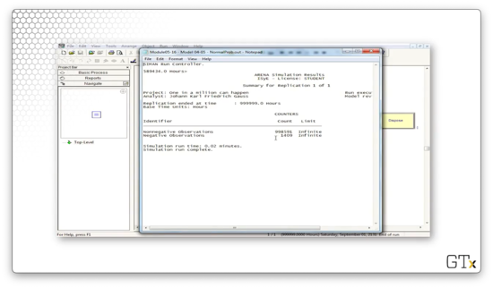
Let's look at the report. Out of the million observations that we generated, 998591 were positive, and 1409 were negative. If we divided each of those numbers by one million, then we have a .9986 probability of seeing a positive Norm(3,1) random variable and a 0.0014 probability of seeing a negative Norm(3,1) random variable. Indeed, the probability of observing a z-score less than or equal to three is 0.0013.
Let's look at another demo. In this example, we are going to use fake customers to generate breakdowns. Here's our setup.
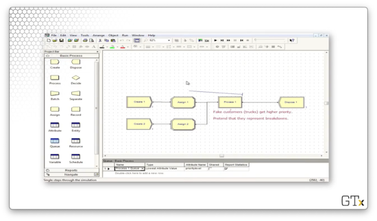
In our first Create block, we create regular customers from an EXPO(0.5) distribution.
In our second Create block, we create fake customers from an EXPO(10) distribution.
We assign two attributes to the regular customers: one named "service time", which takes a value of TRIA(0.5,1,1.5), and one named "priority level", which takes a value of "2".
We assign the same two attributes to the breakdown demons, but with different values: "service time" takes a value of TRIA(3,4,5), and "priority level" takes a value of "1". Note here that these fake customers will jump ahead of normal customers because of their priority levels, and they will take much longer to serve due to their service time distribution.
Now, in the Process block, we see that we serve customers according to the value of the "service time" attribute.
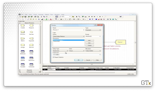
Finally, let's look at the Queue spreadsheet. The queue associated with process one has a Type of "Lowest Attribute Value" and an Attribute Name of "priority level". These configurations ensure that the queue is effectively priority-ordered. For example, a customer with a priority level of one advances ahead of a customer with a priority level of two.
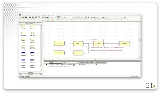
If we run this simulation, we see that the fake customers jump to the front of the line and jam up the system for a long time, which prevents our real customers from being processed.
Advanced Process Template
In this lesson, we will add to our arsenal of modules and spreadsheets by introducing the Advanced Process template.
Advanced Process Template
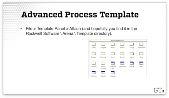
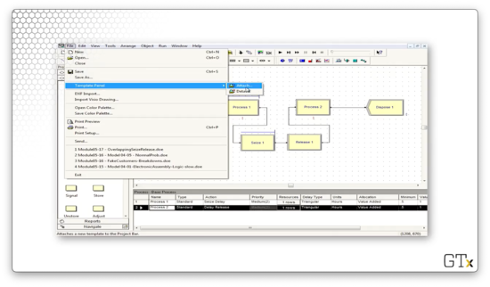
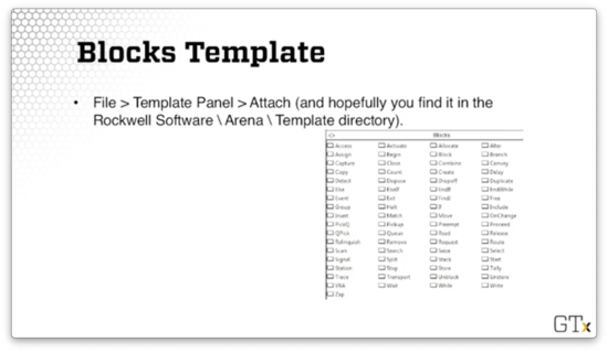
We can access this template by clicking the File > Template Panel > Attach menu option and then selecting the template file from the Rockwell Software\Arena\Template directory on our local machine.
Here's what the template looks like. As we saw in the Basic Process template, this template has several modules and spreadsheets. In the next few lessons, we will focus specifically on the Seize, Delay, and Release modules and the Expression and Failure spreadsheets.
Seize, Delay, Release
Why do we have separate Seize, Delay, and Release modules when we already have these features within the Process module? As it turns out, we often have scenarios that are too complicated for the basic functionality that lives in that module.
Having that functionality split across modules means we can now have setups like Seize, Assign, Delay, and Release, where we assign some attribute after seizing a server.
Furthermore, we can perform non-symmetric seizes and releases. When working in the Process module, we usually released the same resources that we had seized. Now, we can customize our release and only let go of a subset of the resources we seized.
Finally, we use these modules to perform seizes and releases that depend on sets of servers. We will talk about resource sets in the upcoming lessons.
DEMO
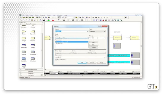
In this demo, we will look at a model that involves Seize and Release as distinct modules. Specifically, we are using separate blocks here so we can perform overlapping seizes and releases. Here's our setup.
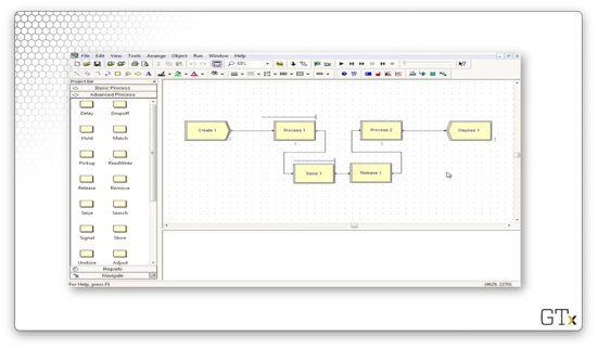
Let's look at this demo in action. Notice that, while we see a line forming behind Process one, we never have a line behind Process two.
In Process one, we perform a Seize-Delay of a resource. The Seize block seizes the resource of Process two, while the Release block releases the resource of Process one. The effect this set up has is that a customer cannot release a Process one resource until a Process two resource is available. As a result, there is no line behind Process two.
If we look at the configuration for the first Process module, we see the Seize-Delay action we just described.
If we look at the Release block, we see that we are releasing Resource 1, the resource we seized in the Process block.
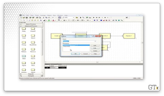
In the second Process block, we perform a Delay-Release on Resource 2, which we seized in the Seize block.
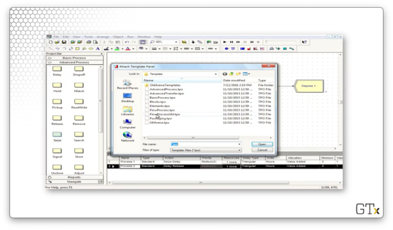
Before we go, let's look at how to import the Advanced Template panel. We start by clicking File > Template Panel > Attach.
We might have to do some hunting, but we should end up in a Rockwell Software\Arena\Template subdirectory on our local machine. Here we can select from several different templates.
Resource Failures and Maintenance
In this lesson, we'll study model breakdowns and maintenance in a much more direct way than the "fake customer" approach we took previously. The idea here is that we will be looking at a particular type of schedule: a failure schedule.
Failures
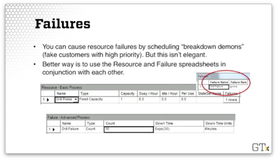
We can cause resource failures by scheduling "breakdown demons" - fake customers with high priority - but this approach is not particularly elegant. The better approach is to use the Resource and Failure spreadsheets in conjunction with each other.
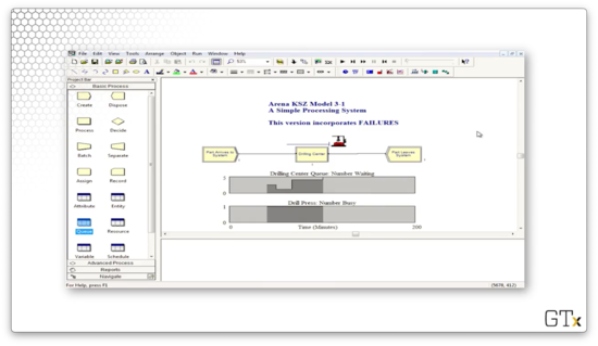
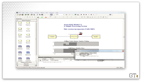
Let's look at a Resource spreadsheet. Notice that the very last column is called "Failures". If we click on the row, we see we have a failure called "Drill Failure".
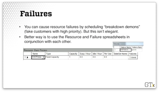
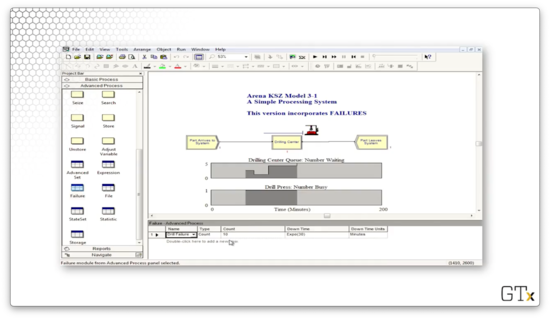
If we head over to the Failure spreadsheet, we can see the "Drill Failure" we just associated with the "Drill Press" resource. This resource has a Type of "Count" and a Count of "10", which means that this resource will fail after ten customers have used it.
Here's the general recipe. First, we go to the Resource spreadsheet in the Basic Process template. Next, we click on the Failures column and add a failure name. We also have to choose the failure rule, which we will discuss shortly. Third, we go to the Failure spreadsheet in the Advanced Process template.
Now we have to choose the type of failure. We can have a "Count" failure, whereby the resource fails after a certain number of arrivals. Alternatively, we could select a "Time" failure, where the resource fails after a certain amount of time.
Finally, we choose the downtime, which describes how long we need to take the server offline for repair. We can use an expression for the downtime, and, in the example above, we drew downtimes from an exponential distribution with a mean of thirty minutes.
Remarks
We can schedule multiple failures by using multiple rows of the Failures column in the Resource spreadsheet. For example, we might want to depict a type 1 and type 2 failure, as well as a scheduled maintenance downtime.
There are different types of failure rules. The "Ignore" failure rule means that we complete the current customer's service and reduce the repair time correspondingly. For example, if the repair time is 60 minutes, and the failure happens while a customer has 10 minutes left of service, the customer finishes service, and the repair time completes in the remaining 50 minutes.
The "Wait" failure rule means that we complete service of the current customer and delay repair. For example, if the repair time is 60 minutes, and the failure happens while a customer has 10 minutes left of service, the customer finishes service. Then the repair time starts, finishing 60 minutes later.
The "Preempt" failure rule means that we stop service of the current customer and complete service after the repair. In the case of our example, that means we resume the customer's service 60 minutes later and finish them at the 70-minute mark.
DEMO
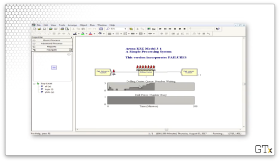
In this demo, we will look at how to use failures. Let's see our setup.
This system contains one resource, a drill press, which has a fixed capacity of one server. We have associated a failure named "Drill Failure" with this resource that has a failure rule of "Ignore".
We can click into the Advanced Process template and look at the Failure spreadsheet to learn more about this failure. As we can see, the failure has a Type of "Count" and a Count of "10", which means that this resource fails after every ten uses. Additionally, the downtime for the drill is sampled from an exponential distribution with a mean of 30.
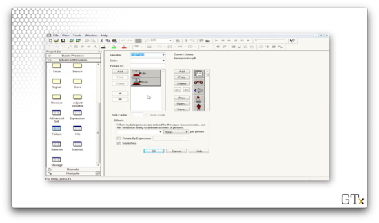
Let's click into the drill graphic. We can see that we have graphics for "Idle" and "Busy", but we don't have a graphic for the failure state. As it turns out, the image will disappear when the drill fails.
Indeed, after we process our tenth customer, the drill press goes away.
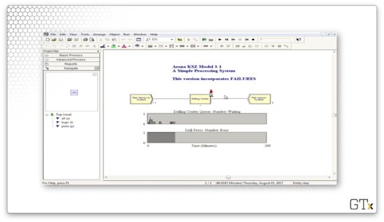
While the drill press is down, the queue begins to grow.
The Blocks Template
In this lesson, we'll add to our ever-growing bag of tricks by learning about the Blocks template.
Blocks Template
Just as we did with the Advanced Process template, we can access the Blocks template by clicking the File > Template Panel > Attach menu option and then selecting the template file from the Rockwell Software\Arena\Template directory on our local machine.
Here's what the Blocks template looks like. There are many blocks in this template, and altogether they sort of form a self-contained language related to SIMAN, the predecessor of Arena.
These blocks are very specialized and low-level, and they offer us much more fine-grained control than the blocks we've seen in the two process templates. We'll only use a few, for now, namely the Seize, Delay, Release, Queue, and Alter blocks.
It might seem strange that we are seeing Seize, Delay, and Release for what feels like the third time in Arena. The main reason for this repetition is that Arena has been built in layers over the years; these concepts have existed and evolved from the SIMAN layer to the current incarnation of Arena.
Additionally, certain primitive blocks, like the Queue block, can't even connect to a Seize module from the Advanced Process template or a Process module from the Basic Process template. For that reason, sometimes we are stuck using blocks from the Blocks template.
DEMO
In this demo, we will look at the use of certain primitive blocks, particularly the Queue block, the Seize block, and the Delay block. Here's our setup.
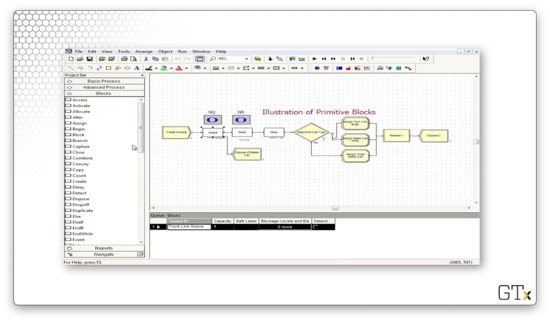
In this example, we create some arrivals, and then we try to seize a resource called "Trunk Line", which represents our bank of telephone lines. If we look at the Resources spreadsheet, we see we have a resource named "Trunk Line", with a Type of "Fixed Capacity" and a Capacity of "3".
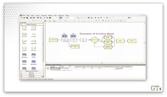
Let's look at the configuration for the Queue block. Notice that we have a Capacity of "4", which means that we will allow four customers in the queue.
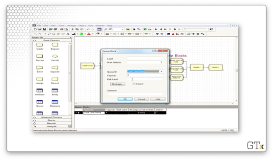
If we head over to the Queue spreadsheet, we see we have a queue named "Trunk Line.Queue" of Type "First In First Out" with a Capacity of "4".
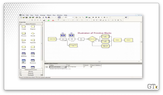
Since the queue only has a capacity of four, customers who arrive after the queue is at capacity are immediately disposed of and removed from the system.
Note that, since we are using the primitive Queue block, we have to attach it to a primitive Seize block, which we follow up with a primitive Delay block.
We also maintain counters for the number of people in the queue and the number of servers being used above the Queue and Seize blocks, respectively.
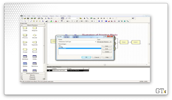
After the resource is seized and delayed, the customers enter into a Decide block that makes a "3-way by Chance" decision. The customer will follow the first branch 76% of the time, the second branch 16% of the time, and the third branch the remaining 8% of the time.
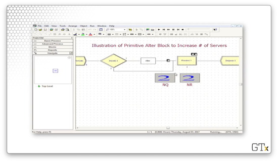
Let's look at another demo. In this example, we use an Alter block, which is responsible for adding servers to or subtracting servers from a resource. Here's our setup.
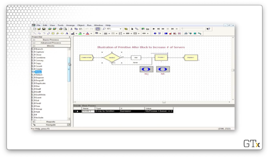
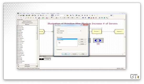
Let's look at the configuration for this Alter block. This block has an entry under Resources called "Barber, 1", which means that we increase the number of servers in the "Barber" resource by one every time we pass a customer through the block.
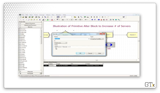
Let's look at the configuration for the Decide block that precedes the Alter block. Here we see that we have a "2-way by Condition" decision that evaluates the expression NQ(Process 1.Queue) >= 3. In plain English: if the number of people in the queue behind Process 1 is greater than or equal to three, the expression is true, and we pass the customer through the Alter block and add a server.
Additionally, we keep track of the number of people in the queue and the number of currently working servers.
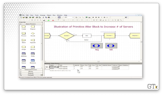
Let's head over to the Resource spreadsheet and see how many servers we have at the beginning of the simulation. We can see that for the "Barber" resource, we have a fixed capacity of one server.
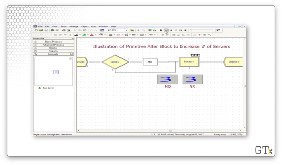
Let's step through the simulation. At one point, we have a queue size of three, with one server in use by a customer.

At this point, the fifth customer passes through the alter block and causes the Barber resource's capacity to increase by one. The extra barber grabs someone from the line and starts serving them, resulting in two working barbers and two queued customers.
When the sixth customer arrives, the queue size is back at three, so he also enters the Alter block and bumps the capacity up to three. As a result, after he joins the queue, three customers are in the queue, and three customers are in service.
The Joy of Sets
In this lesson, we're going to learn how to use sets to enhance our modeling abilities. We'll primarily concentrate on resource sets.
Sets
A set is just a group of elements. Elements are allowed to belong to more than one set. Elements can be anything in Arena, and, as a result, Arena has many different types of sets, such as:
- Resource Sets
- Counter Sets
- Tally Sets
- Entity Type Sets
- Entity Picture Sets
Resource Sets
We can use the Set spreadsheet in the Basic Process template to define sets. So far, the "vanilla" resources we have created have identical interchangeable servers. If we have a resource that has five barbers, those barbers all look and act the same, and we don't care which is which.
A resource set can have distinct servers, each with different schedules, service speeds, and service specialties. In fact, a resource set is much more general and powerful than the simplistic resources we have been working with until now.
Call Center Example
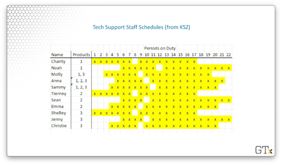
In our call center example, we'll have three products with the following resources. If we have a question about product one, we'll talk to Charity, Noah, Molly, Anna, or Sammy. If we have a question about product two, we'll talk to Tierney, Sean, Emma, Anna, or Sammy. If we have a question about product three, we'll talk to Shelley, Jenny, Christina, Molly, Anna, or Sammy. All eleven servers have distinct schedules.
Notice that several servers exist in multiple sets; in other words, they have a degree of cross-functionality. We've listed these servers at the end because, in Arena, we can order sets, and we reserve the most talented servers for last, so we don't waste them if we don't need to.
Back to Resource Sets
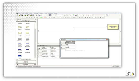
Let's say we want to define a resource set called "Product 1". To accomplish this, we first go to the Set spreadsheet and select "Resource" from the Type dropdown. Next, we click into Members and then enter the appropriate servers under Resource Name.
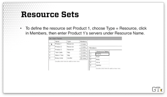
Note that this list of resources is ordered such that when we draw a member from this set, we try to select Charity first, then Noah, and so on. As we said, we save Sammy for last because he is cross-functional. We can also define other ordering schemes.
Seize-Delay-Release
When we perform a Seize-Delay-Release with a server in a resource set, we must be cautious. The problem is that we have to make sure that we release the same server that we initially seized. If we release a random server, we might be stopping service on some other customer.
Let's walk through how we might seize a server from the product one set and then release that same server, using the Seize, Delay, and Release blocks from the Blocks template.
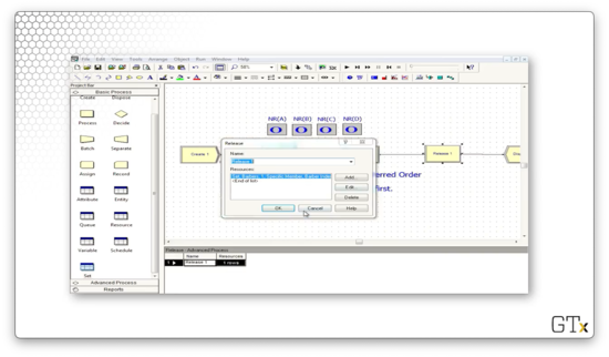
Let's look at the configuration for the Seize block first. As we can see, we are seizing from a Type of "Set", where the Set Name is "Product 1". We are seizing one server from this set - Quantity equals "1" - and we are using "Preferred Order" as the Selection Rule. Finally, we are saving the server's index in the set as an attribute called "Tech Agent Index" on the seizing customer.
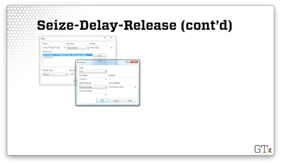
Now let's look at the configuration for the Release block. Here we are releasing one server from the Product 1 set. In this case, the Release Rule is "Specific Member", and we are releasing the server whose index in the set is equal to the "Tech Agent Index" attribute on the customer, which we set when the customer seized the server.
Remarks
Various seize selection rules are possible. We can seize servers in a cyclical fashion, ensuring that we don't tire out any one server before the others. Alternatively, we can seize servers randomly. We can also seize servers according to the preferred order like we are doing here, or we could seize a specific member.
We can seize according to the resource with the largest remaining capacity. For example, if there are more manicurists available than barbers, we could seize a manicurist. As well, we could seize the resource with the smallest number of busy servers.
DEMO
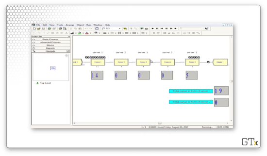
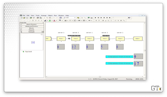
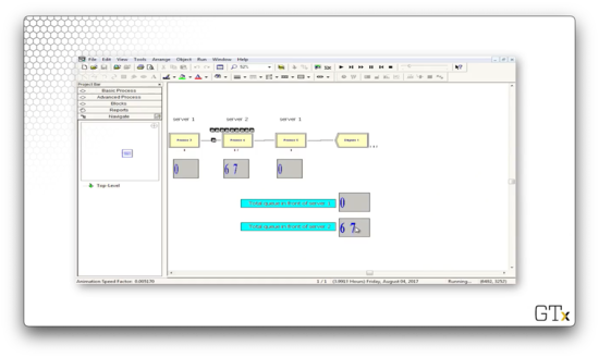
In this demo, we will look at how to use resource sets. We have four servers associated with a particular resource - A, B, C, and D - and we'd like those servers to be seized in that order. Specifically, resource B should only be seized if A is busy, and resource C should only be seized if B is busy, and so on.
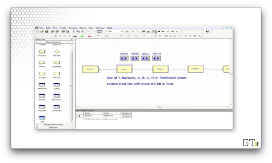
Let's look at the this demo in action. Notice how we always try to fill the leftmost zero as the simulation proceeds.
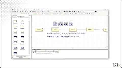
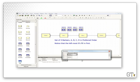
We can head over to the Set panel and see that we have a resource set named "Barbers" that has four rows, one each for barbers A, B, C, and D.
Now let's look at the language we have to use in the Seize and Release blocks to emulate this preferred order behavior appropriately.
In the Seize block, we can see that we are seizing one barber from the "Barbers" set. We seize the servers in preferred order, and we set the index of the server as an attribute called "Barber Index" on the seizing customer.
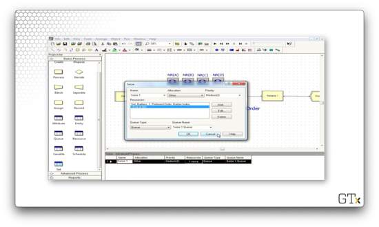
Let's see how we configure the Release block. Here, we are releasing one specific member of the "Barbers" set. Which one? We look at the "Barber Index" attribute on the customer and release the server whose index in the set equals that attribute's value.
Description of Call Center
In this lesson, we will talk through the call center example in plain English.
Call Center Description
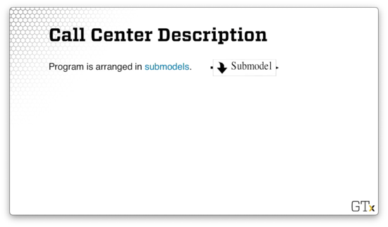
First of all, the program is arranged in sub-models. A sub-model is basically a subroutine that undertakes a specific task in the program that would otherwise take up a lot of space. Here is how we represent a sub-model in Arena.
We will use one sub-model to create and direct arrivals, which will serve the purpose of helping us simulate how often calls show up and how calls get routed.
We also have a tech support sub-model where we handle all of the tech support calls. As it turns out, we will have three different types of products in this model, and customers need to be served by tech support representatives with the appropriate product knowledge. Additionally, some of the tech support calls require return calls, so we have another sub-model encapsulating this callback functionality.
We also have sub-models for sales calls, and order status calls - "Has my order shipped yet?" - as well as a time period counter sub-model. This last sub-model allows us to understand which 1/2-hour period of the day we are currently in.
Arrivals
The call center accepts calls from 8 AM to 6 PM, and calls show up during this period according to a nonhomogenous Poisson process whose arrival rate changes every half hour. Here are the call arrival rates throughout the 20 half-hour increments. Be careful: the rates below are hourly rates, even though they change every half-hour.
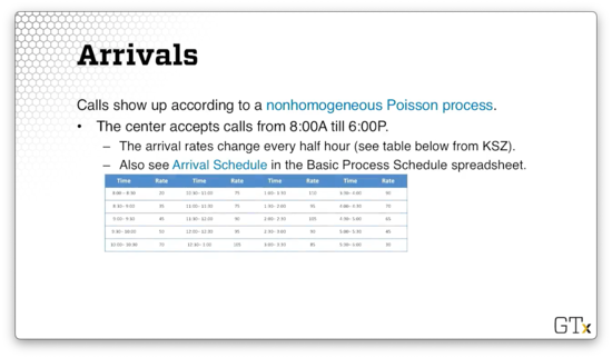
A few staff stay at work until 7 PM in order to let the calls at the end of the day clear out. Given that there are no calls between 6 PM and 7 PM, we have to explicitly model zero arrivals for those two half-hour segments.
Phone Lines
There are 26 phone lines. If a customer receives a busy signal, they immediately get disposed. We will associate a Queue block with capacity zero with a Seize block that attempts to seize a phone line. If the Seize fails, there's no queue to enter, so the customer leaves the system.
Remember that the Queue and Seize blocks both come from the Blocks template panel. This panel is the only place where we can find a Queue block, and this block only connects to this type of Seize. We cannot connect a Queue block to a Seize block from the Advanced Process template or a Process block from the Basic Process Template.
Types of Calls
There are three general types of calls, which we'll handle with an "N-way by Chance" Decide module. Each customer hears a telephone recording for a UNIF(0.1, 0.6) amount of time while they make their choice. 76% of the customers go to tech support.
Additionally, 16% of customers go to sales. Sales consists of seven identical, interchangeable resources. In other words, while the tech support servers are part of a resource set, sales is a vanilla type of resource that we have worked with often before. Sales calls take a TRIA(4,15,45) amount of time.
Finally, 8% of the customers go to order status. 85% of these customers can self-serve in a TRIA(2,3,4) amount of time, but 15% need to talk to a sales representative for a TRIA(3,5,10) amount of time.
Tech Support
There are three different types of tech support calls, which we'll again handle via a Decide module. 25% of customers need support for product one, 34% for product two, and 41% for product three. Each customer hears another recording for a UNIF(0.1,0.5) amount of time while they make their choice.
All tech support calls require staff for a TRIA(3,6,18) amount of time. We could make each type of call require a different amount of time, but we've had enough complexity thus far.
Call Backs
Tech support may not be able to handle a customer's call right away, and 4% of tech support calls require additional investigation and a callback. Another group of staff, which we won't worry about, carries out this investigation. The customer's original server is freed up when he or she determines that more research is needed.
This investigation takes an EXPO(60) amount of time. After the investigation is complete, the original tech support server will call the customer back using one of the 26 available phone lines with high priority. That return call takes a TRIA(2,4,9) amount of time.
Tech Support Info
The tech support staff work for 8-hour days with thirty minutes for lunch, and every server has a different schedule. Additionally, the support staff all have different product expertise. Here are the preferred orders for servers on a per-product basis:
- Product 1: Charity, Noah, Molly, Anna, Sammy
- Product 2: Tierney, Sean, Emma, Anna, Sammy
- Product 3: Shelley, Jenny, Christie, Anna, Sammy
Here is the schedule for the various tech support staff. As we can see, everyone works at different hours and has different break times.
Call Center
In this lesson, we will put together many different ideas from the recent lessons. We will combine everything we learned, from fake customers to resource sets, to simulate a complex call center.
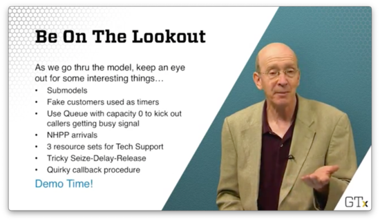
Be On The Lookout
As we walk through this model, let's look out for many of the different components that we talked about so far.
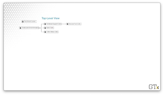
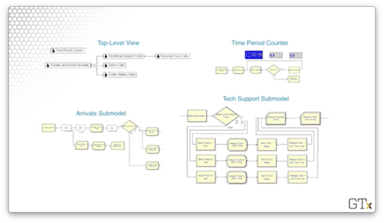
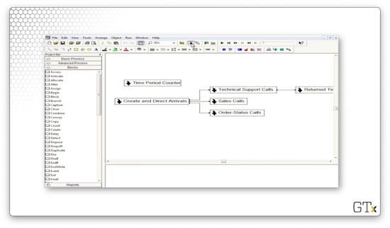
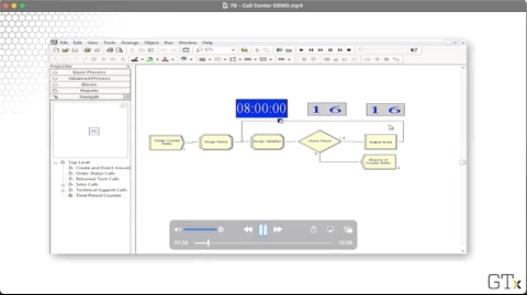
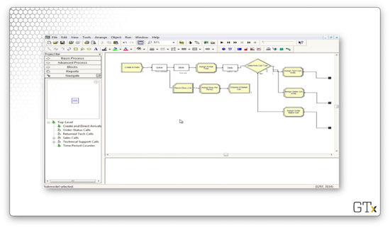
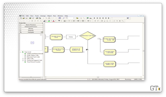
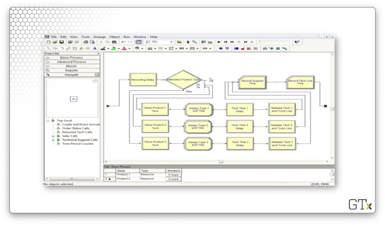
Here is the top-level view of the overall model, which displays the sub-models.
Here are the Tech Support sub-model, the Time Period counter, and the Arrivals sub-model.
DEMO
Here's the main screen for the call center. As we can see, it's arranged into sub-models. We can create a new sub-model by clicking on the arrow icon in the main toolbar.
Notice the connections between the various sub-models. The Create and Direct Arrivals sub-model connects to the Technical Support Calls, Sales Calls, and Order-Status Calls sub-models. In turn, the Technical Support Calls sub-model connects to the Returned Tech Support Calls sub-model. The Time Period Counter sub-model does not connect to any of the other sub-models.
Let's look at the Time Period Count sub-model. Here's our setup.
This submodel's only job is to use fake customers to update the time period. Every eleven hours, we create a new fake customer, and every half hour, this customer updates a variable called "period". This variable is useful for certain statistics gathering, as well as keeping track of when the arrival rate changes and when the servers go on break.
When the counter hits twenty-two, we dispose of the fake customer, reset the counter to zero, and generate a new timekeeper. Note that the clock starts at midnight, not at 8 AM, when the call center opens. Using the period variable instead of the absolute time to keep track of the day, we can pretend that the clock runs from 8 AM to 6 PM.
Now let's look at the Create and Direct Arrival sub-model. Here's our setup.
Let's look at the first piece. We create customers, and then those customers enter into a queue of capacity zero while attempting to seize a resource called "Trunk Line", which has 26 servers. If all trunk lines are busy, the customers enter into the queue, but since the queue has capacity zero, they are immediately kicked into the "Record Busy Line" Record block. We gather some statistics, and then we dispose of the customer.
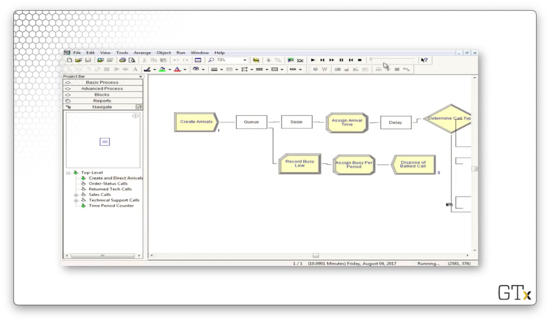
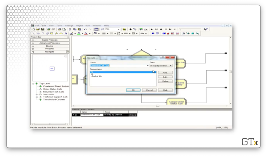
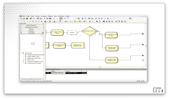
If the customer can seize a trunk line, we assign the arrival time, play some music for the customer in a Delay block, and then enter a Decide block to determine the customer's call type.
Let's look at the Decide block. As we can see, we have an "N-way by Chance" decision where we select the tech support branch 76% of the time, the sales branch 16% of the time, and the order branch 8% of the time, just as we specified earlier.
After we determine the type of call, we are done with this sub-model. We can see the small, black, square terminals at the end of each branch, indicating that we need to return to the main program.
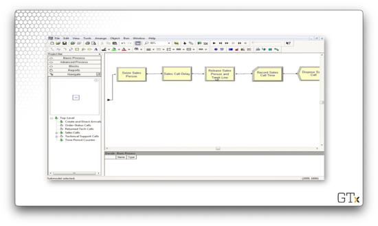
Now, let's turn the Sales Call sub-model. Essentially, the customer seizes a salesperson, waits for some time, and then releases the salesperson and the trunk line. Finally, we collect some call statistics and then dispose of the caller. Here's our setup.
Let's take a look at our resources in the Resource spreadsheet. Here we see our individual tech support staff and our nameless, faceless sales support staff. Additionally, we see our Trunk Line resource with its fixed capacity of 26.
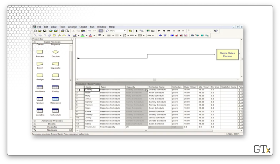
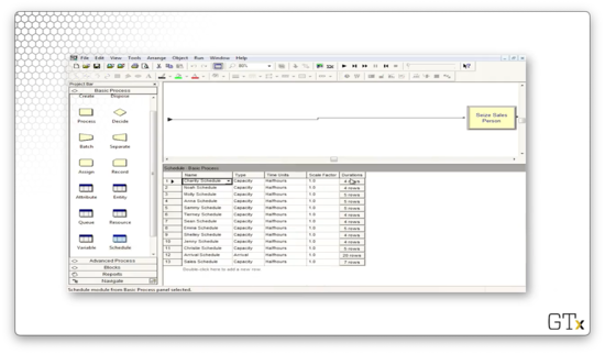
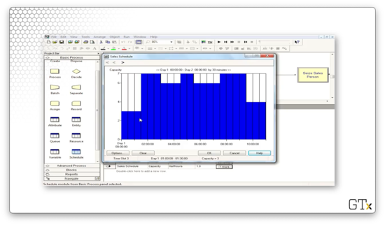
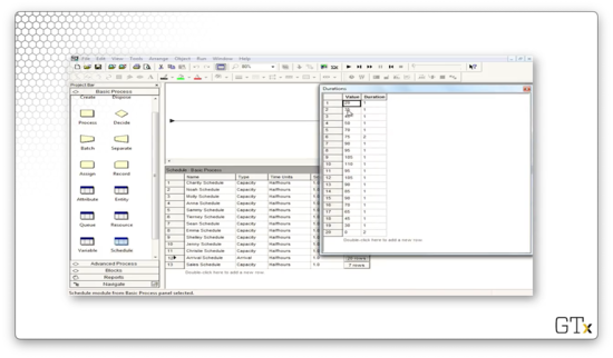
Let's take a look at the Schedule spreadsheet so we can see the schedules of our various employees.
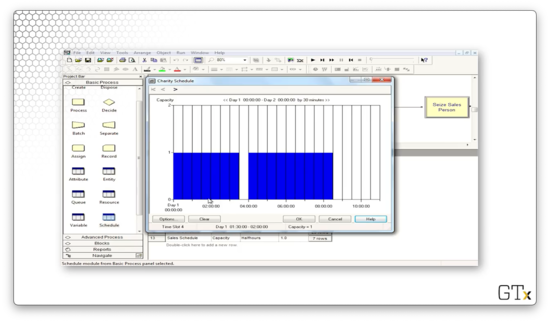
Here's Charity's schedule. We can see that she works for three and a half hours, takes a lunch break, works for another four and a half hours, and then goes home.
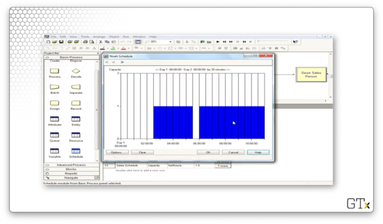
Now let's look at Noah's schedule. He works later, starting two and a half hours into the day and working until the call center closes.
We can look at the schedule of the sales servers. Notice that throughout the day, the capacity of this resource varies between three and seven servers.
Finally, we can look at the call arrivals schedule. Notice that this schedule has a Type of "Arrival" instead of "Capacity". This arrival schedule starts small, peaks in the middle of the day, and falls off towards the end of the day. The final two half-hour segments have zero arrivals. This period corresponds to the call center's closing hour when employees are wrapping up calls that began before 6 PM.
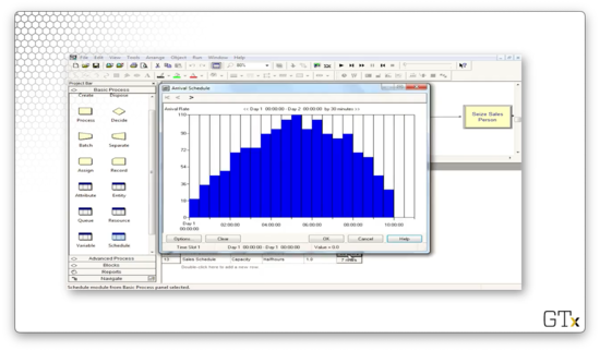
While we can edit the schedule by clicking on the bars themselves, we can alternatively right-click on the "rows" button for the associated schedule and select "Edit Spreadsheet" to edit the schedule more easily. We can set the same arrival rate for two time periods by setting the corresponding "Duration" cell to "2".
Again, remember: the arrival rates are per-hour rates, while the time periods are half-hour segments.
Now let's turn to the Set spreadsheet. If we click into the "Product 1" set, we see the employees that can assist with product one, listed in the preferred order.
Similarly, if we click into the "Product 2" set, we see the employees that can assist with product two, listed in the preferred order.

Now let's turn to the Tech Support Calls sub-model. Here's our setup.
Each customer first experiences a Delay where they listen to a recording before randomly choosing one of the three product types. Once they choose their product type, they seize the appropriate support server for that product.
Next, the customer encounters an Assign block where they are assigned an attribute corresponding to their product type as well as an attribute marking the time the call starts. Then, they delay their tech support rep for a random amount of time, after which they release both the rep and the trunk line.
Let's walk through the flow for a customer receiving tech support for product one.
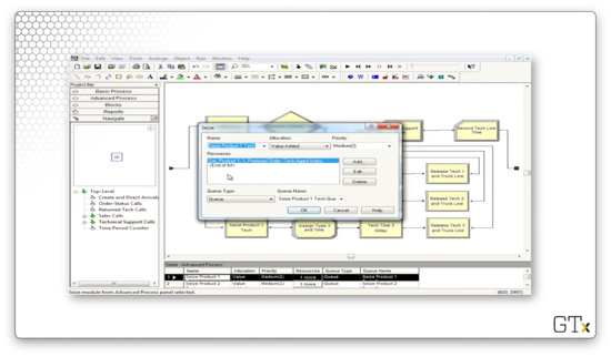
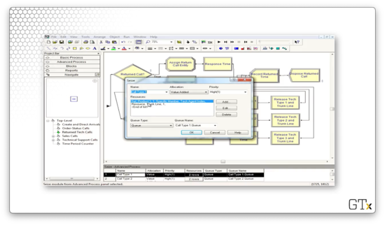
Let's look at the configuration for the Seize block. As we can see, we are seizing one server from the Product 1 resource set in the preferred order. We store the index of the server we seize as an attribute called "Tech Agent Index" on the seizing customer.
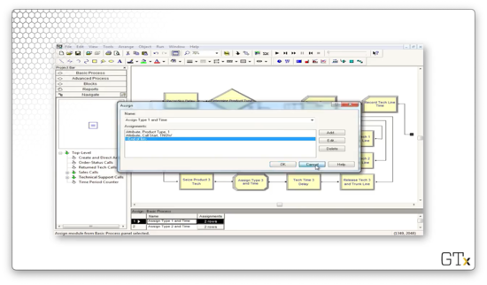
Let's look at the configuration for the Assign block. We set an attribute called "Product Type", which has a value of "1" and an attribute called "Call Start" which has a value of TNOW.
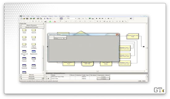
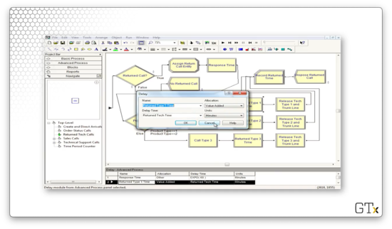
Now let's look at the configuration for the Delay block. Notice that we delay the server according to an expression called "Tech Time". We extract this value out into an expression because we use the same service time for each type of tech support call.
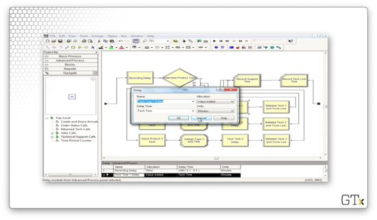
If we head over to the Expression spreadsheet and select the "Tech Time" expression, we can see that it refers to a TRIA(3,6,18) distribution. Thus, our service times come from this distribution.
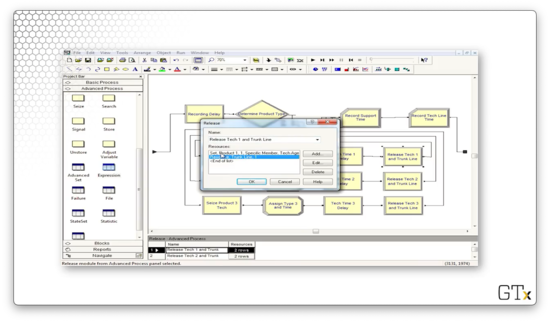
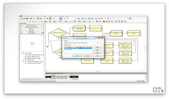
Finally, let's look at the configuration for the Release block. Here we release one member of the Product 1 resource set, specified by the value of the "Tech Agent Index" attribute stored on the customer. Additionally, we release the trunk line.
If we run the simulation, we might notice that all of the customers who pass through the Tech Support Calls sub-model also pass through the Returned Tech Calls sub-model. Let's look there next. Here's our setup.
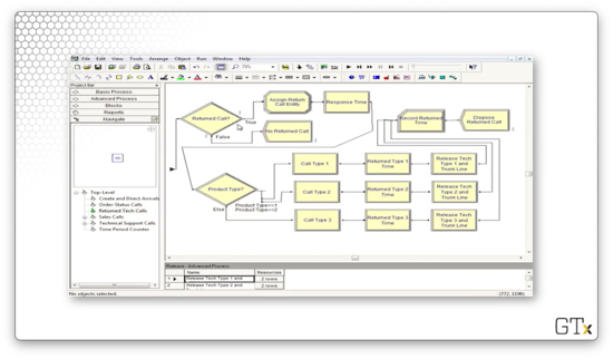
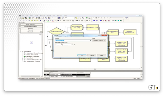
Even though every customer enters this sub-model, only 4% of the customers actually traverse the callback flow, while 96% are immediately disposed. As we can see, the Decide block right at the front of this sub-model makes that decision.
The customers who require a callback encounter another Decide block, which reads off the "Product Type" attribute we set back in the Tech Support Calls sub-model. The Decide block uses this attribute to route the customer to the appropriate callback progression.
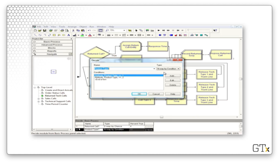
How do we emulate a callback? We can use a Seize block configured to seize a trunk line and the product support server from the appropriate resource set with high priority. Note that, technically, the customer is calling in to the system, but, since the priority is set to high, they will immediately get their server when they become available. This configuration effectively resembles the employee calling out to the customer.
Also, note that we retrieve the same server we spoke to before, as referenced by the "Tech Agent Index" attribute. We do not seize the server by preferred order as we did in the previous sub-model.
We then delay the agent according to the "Returned Tech Time" expression.
Finally, we release that particular agent and the trunk line.
The last component we have to look at is the Order-Status Call sub-model. In a nutshell, customers enter this flow, receive some delay, and then take one of two paths. They either perform a Seize-Delay-Release with a salesperson followed by a Record and Dispose, or immediately flow through the Record and Dispose. Here's the setup.
An Inventory System
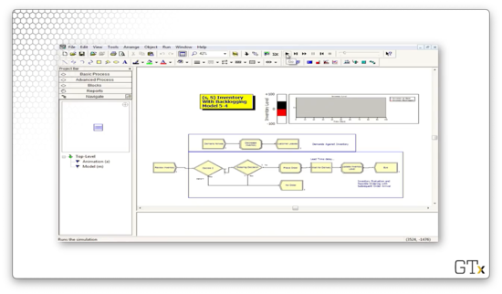
In this lesson, we will give a plain-English description of an (s, S) inventory system, followed by a demo in Arena.
Description of (s, S) Policy
Here we will simulate the inventory stock of a widget over time using modules from both the Basic and Advanced Process templates.
We generate customer interarrival times via an EXPO(0.1) distribution, so we receive about ten customer arrivals per day. We generate the demand size from a discrete distribution, which we specify with the DISC command. We always meet demand; even if we don't have the inventory on hand, we never turn a customer away.
We "take" (evaluate) inventory at the start of each day, and this is the only time we can notice that we are under-stocked. As per (s, S) semantics, if the inventory is below 's', we order up to 'S'. For example, if 's' is 5, and 'S' is 20, and we start the day with an inventory of 4, we place an order for an additional 16 units.
We generate delivery lead times from a UNIF(0.5,1) distribution, which means that we receive stock between half a day and a full day after ordering it. This timing is quick, but, by the time the order arrives, other customers will have also arrived, depleting inventory further.
We have multiple costs. First, there are order costs: we pay a flat cost every time we place an order and a unit cost per item. Additionally, we have holding costs - cost on unsold inventory that sits overnight - and penalty costs, which we pay when customers demand more inventory than we have. Using all these various costs, we want to calculate the average total cost per day over 120 days.
Inventory, unit costs, and all of the other parameters are Arena variables. We decrement inventory when demands arrive and increment it when orders arrive, and we take inventory using a "fake" customer at the beginning of each day. Interarrival times, demands, and lead times are all expressions from the Advanced Process template. We also use the Advanced Process template to calculate accumulated costs via the Statistic spreadsheet.
DEMO
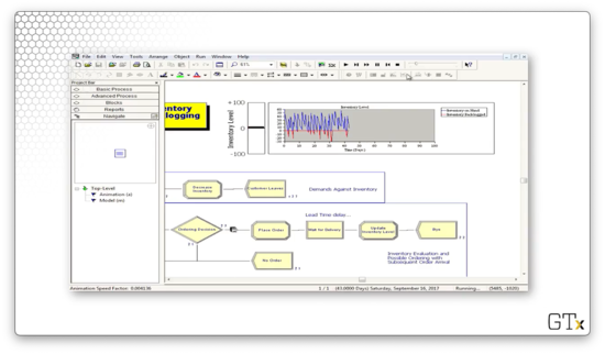
In this demo, we are going to look at an (s, S) inventory system. Here's our setup.
Let's zoom in on the customer arrivals. Customers arrive according to an expression called "Interdemand Time", decrement the inventory according to a discrete distribution, and then leave.
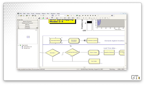
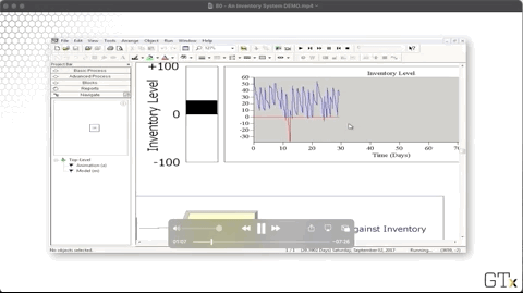
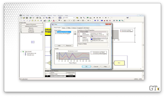
We plot the system's inventory using an inventory level fill bar and a corresponding histogram in the upper-right corner of the main workspace area. As we can see, we rarely dip into the red - inventory below zero - and we experience the sawtooth pattern of declining inventory followed by large orders.
We can look at the Assign block that newly created customers pass through to see how each customer decreases inventory. We are updating a variable called "Inventory Level" to the value "Inventory Level - Demand Size", where "Demand Size" is an expression.
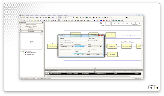
Once a day, we create a fake customer to review the inventory. This customer arrives according to an expression called "Evaluation Interval".
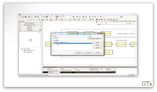
Sometimes this fake customer places an order. Let's take a look at the first of two Decide blocks in this flow. This block makes a "2-way by Condition" decision based on whether a variable called "ongoing" is equal to "0". This variable refers to whether the previous order is complete. If so, the customer proceeds to the next block; otherwise, they exit the system.
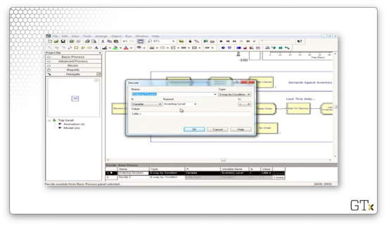
Let's look at the second Decide block, which determines whether we place an order. Here we have a "2-way by Condition" decision, which is true if the variable "Inventory Level" is less than the variable "Little s". If so, we place an order; otherwise, we exit.
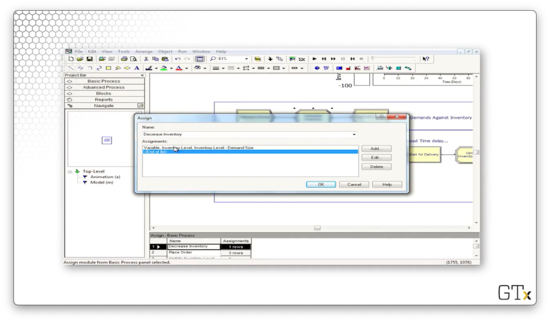
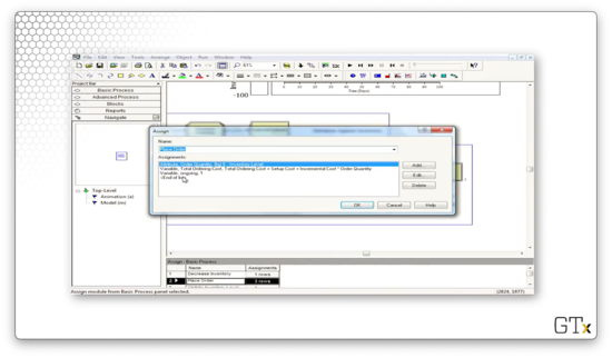
Assuming we place an order, we head next to an Assign block. Here, we update an attribute called "Order Quantity" to the value of "Big S - Inventory Level". Additionally, we update a variable called "Total Ordering Cost" to the value of "Total Ordering Cost + Setup Cost + Incremental Cost * Order Quantity". Finally, we set the "ongoing" variable to "1" to ensure that we don't place multiple orders within two days.
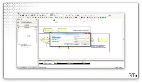
Next, we enter a Delay block as we wait for our order. Here, we wait according to the expression "Delivery Lag".
After the delivery occurs, we enter another Assign block. Here we set the variable named "Inventory Level" to "Inventory Level + Order Quantity", and we set the variable "ongoing" to "0", so we can place orders again in the future.

Let's look at the configuration for the inventory level chart. Notice that our "Inventory on Hand" line corresponds to the expression "MX(Inventory Level, 0)", where "MX" refers to the max. There is another expression that produces the "Inventory Backlogged" line chart (the red one).
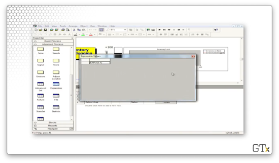
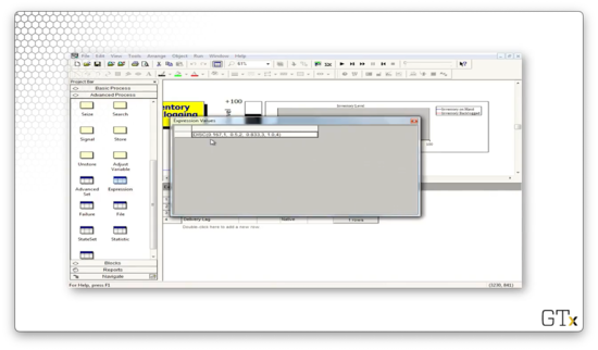
Let's look at some of the expressions we have in the Expression spreadsheet in the Advanced Process template panel. The "Interdemand Time" refers to an EXPO(0.1) distribution.
The "Demand Size" expression refers to a DISC(0.167,1,0.5,2,0.833,3,1.0,4) distribution. Looking at this distribution, we can see that we generate the value "1" with probability 0.167, the value "2" with probability 0.333, the value "3" with probability 0.333, and the value "4" with probability 0.167.
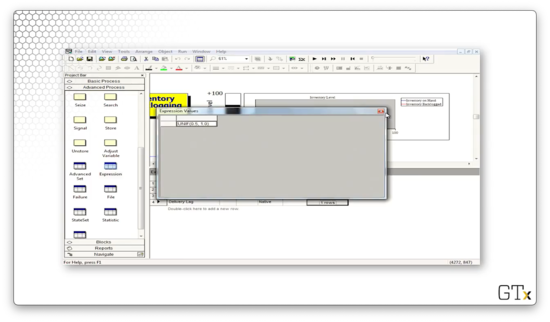
The "Evaluation Interval" expression takes a value of "0.5", which means our fake customer checks the inventory levels twice per day. With such frequent monitoring, it's no surprise our inventory rarely dips into the red.
Finally, the "Delivery Lag" expression takes a value of UNIF(0.5,1.0).
We have several variables that we maintain, and we can check those out in the Variable spreadsheet in the Basic Process template panel. For example, we could click into "Little s" and "Big s" and uncover that we are simulating a (30, 60) inventory system.
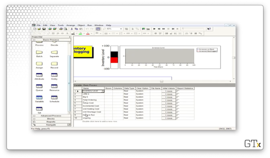
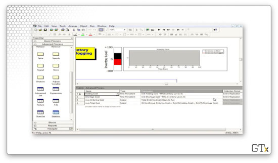
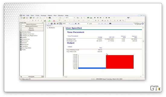
Let's go back to the Advanced Process template panel and look at the Statistic spreadsheet, which keeps track of our various costs: holding cost, shortage cost, average ordering cost, and average total cost.
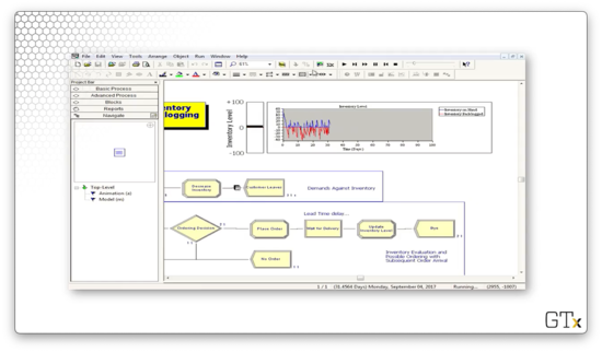
Let's see what happens when we change the value of the "Evaluation Interval" expression from 0.5 to 1.0. This change cuts our monitoring frequency in half, and, as we might expect, we find our inventory in the red a lot more often.
Let's see what happens if we drop "Little s" from 30 to 10 and drop "Big S" from 60 to 30. In this case, we are waiting right until we run out of inventory to restock, and, on top of that, we are monitoring too infrequently. As a result, we see a lot of red.
Let's look at some reports. The main variable that we care about is "Avg Total Cost", which refers to how much we have to spend daily to keep the shop running. In this case, we have to spend just under $143.
One Line vs. Two Lines?
In this lesson, we will ask the question: should we use one line feeding into two parallel servers or two lines feeding into two individual servers? We'll use a technique called common random numbers to make an apples-to-apples comparison.
Game Plan
We have two options to explore. In option A, customers show up and join one line in front of two identical servers, selecting whichever server is available first. In option B, customers randomly choose which of two lines - in front of single servers - to join.
We will compare which of A or B is better by using the exact same customers - really, the same customer arrivals - and we'll use a Separate module to duplicate the customers before sending them off to each option. Additionally, each customer will receive the same service time regardless of whether they use option A or B, and we'll enforce this consistency with an early Assign module.
We are going to assume that, almost certainly, option A is better. In option B, it may be the case that a customer randomly chooses not to use a server with an empty line.
Using the same arrival and service times for both experiments - the common random numbers technique we mentioned at the start of the lesson - sets the stage for easy apples-to-apples statistical comparison.
DEMO
Now we are going to demo this one-line vs. two-line problem. Here's our setup.
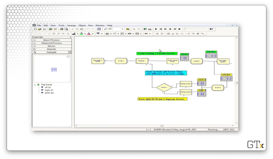
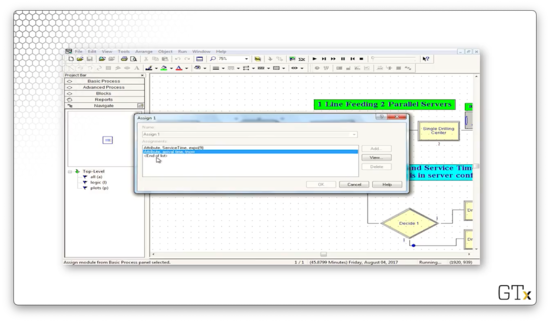
After we create our customers, we assign them an attribute called "arrival time", which takes the value TNOW: the internal variable that Arena maintains that refers to the current time. Additionally, we assign them an attribute called "ServiceTime", which we pull from an EXPO(9) distribution.
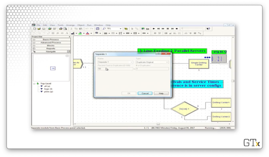
We then split the customer into two clones using the Separate block. We can see the following configuration, which specifies a Type of "Duplicate Original", and that the # of Duplicates is "1". This way, we can send identical clones of the customer to each of the two pathways.
Here are the two pathways that each customer takes.
For the two-queue path, let's look at the Decide module. As we might have guessed, this block specifies a "2-way by Chance" decision where the Percent True field is set to "50%". This configuration corresponds to customers entering one of the two lines at random.
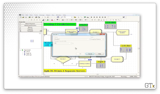
The only other difference between the two paths is that the single Process block in the one-queue path has a capacity of two, while each of the two process blocks in the two-queue path has a capacity of one.
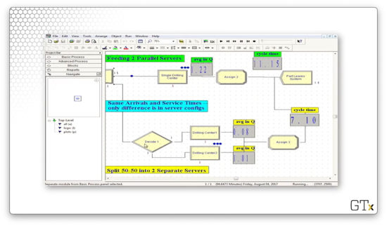
Let's run the simulation for some time and see what happens. After about 5000 minutes, the one-queue pathway has an average cycle time of 21.16, while the two-queue pathway has a cycle time of 47.28. Additionally, the average number of customers in the single queue is about 2.4, whereas the average number of customers in the two queues is 3.3 and 4.2.
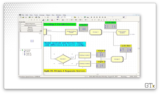
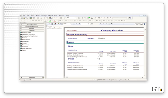
Let's run the simulation to completion and look at the output. We can see that the single-queue drill center has an average waiting time of 41 minutes, whereas the double-queue drill center has average waiting times of 81 and 128 minutes.
Given these statistics, option A is the clear winner.
A Crazy Re-entrant Queue
In this lesson, we will look at a model of a re-entrant queue. As it turns out, when we have customers with changing priorities that re-use servers, we see some very non-intuitive outcomes.
Re-entrant Queues
In this example, customers will visit server one, followed by server two, server one, server two, and finally server one again. We call the queues associated with these servers "re-entrant" because customers re-enter them after receiving service. We depict this flow in Arena with five separate Process modules, each with a Seize-Delay-Release trio that grabs the appropriate server. As a reminder, it is legal to seize the same server in different Process modules.
All service times are exponential. Here are the means:
- 1 (0.1)
- 2 (0.5)
- 1 (0.1)
- 2 (0.1)
- 1 (0.5)
Here are the customer priorities:
- 1 (low)
- 2 (high)
- 1 (medium)
- 2 (low)
- 1 (high)
For example, on the customer's third visit to server one, he has a high-priority EXPO(0.5) service time.
DEMO
Here's our demo setup in Arena. As we said, we create customers every once in a while, and then we pass them through server 1, server 2, server 1, server 2, and server 1 again with varying service times and priorities. Note that, for each server, we keep track of the current queue size. Additionally, we keep track of the total queue length behind server 1 and server 2.
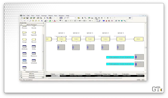
Let's look at the configuration of the first Process block. Here we see that we are seizing the "Server1" resource for an EXPO(0.1) amount of time with a customer priority of "Low". The remaining Process blocks are configured according to our description above.
When we start the demo, we don't see too much activity. After some time, the queues start to grow. At one point, server one has large queues while server two has no queues.
A short while later, the setup flips: server two has large queues, and server one has no queue.
The oscillating behavior that we see results from the careful configuration that we set in the Process modules. We can see that, as time goes on, not only does the oscillation continue, but it gets worse. Towards the end of the demo, we can see upwards of 70 customers in one server's queue while the other queue is empty.
SMARTS and Rockwell Files
In this lesson, we will look at SMARTS files and Rockwell demos. As a reminder, Rockwell is the company that develops Arena.
SMARTS + Rockwell Demos
SMARTS files are tutorial files, organized by subject area, that can occasionally help us with difficult problems when Arena's basic help menus fail us. For example, there's a SMARTS file to create customers with a time-dependent arrival rate that varies according to an equation. There are hundreds of SMARTS files. Rockwell also has prepared many professional demos. To find these resources, we can look in the Libraries > Documents > Rockwell Software > Arena directory path, although the exact location may differ from machine to machine.
DEMO
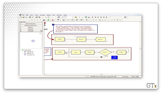
In this demo, we will look at an arrival rate that varies by an expression, which incorporates a variable that changes depending on the day of the week. Here's our setup.
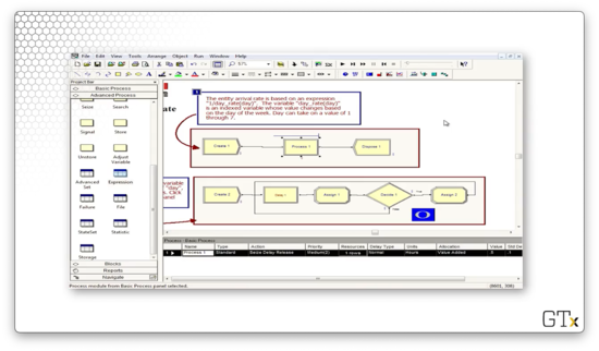
Here's the configuration for our Create block. Notice that we have selected "Expression" from the Type dropdown, and we are using the expression 1/(day_rate(day)) to generate the interarrival times.
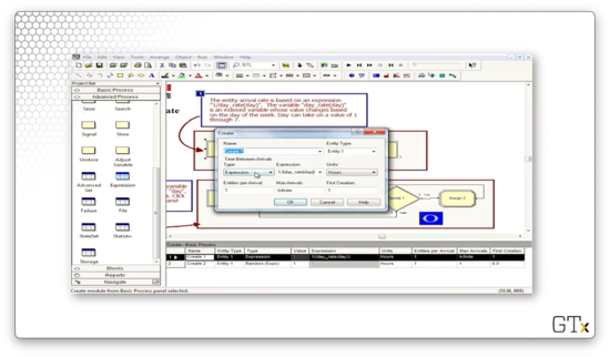
Let's check out the "day" variable in the Basic Process template. This variable holds the current day of the week and is initialized to "1".

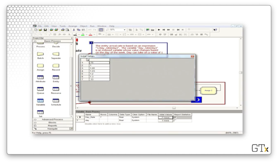
Now, let's look at the "day_rate" variable. This variable is a vector with seven elements, one for each day of the week.
How do we know what day it is? Look at the second row of the model. Every 24 hours, we generate a customer that updates the "day" variable. Thankfully, the program is smart enough to wrap the counter back to "1" after "7".
Note that we didn't have to build this model ourselves; rather, this model comes from one of the hundreds of SMARTS files that Arena provides for us.
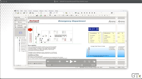
Additionally, Rockwell gives us many excellent demos. Here's a demo of patient flow through and emergency room, which keeps track of various conditions and utilizations.
A Manufacturing System
In this lesson, we'll look at a sophisticated manufacturing cell, along with several variations involving transporters and conveyors. The idea here is to introduce movement and multiple part paths, both of which are extremely useful features that generalize to many different applications.
Description
We have a manufacturing cell that produces three different types of parts, and each part follows a different path, or sequence, through the system. Different service times occur at each station, depending on the part type and the place in the visitation sequence. For example, part two might visit stations 1, 2, 4, 2, and 3, and it will experience different service times for each visit, including the two visits to station two.
Product movement requires the Advanced Transfer template. Once we load it, we will have access to the Route, Station, Enter, and Leave modules, along with the Sequences spreadsheet. This spreadsheet keeps track of the set of paths that the customers - really, parts in this example - can undertake. We'll need advanced sets to handle sets of sequences.
Parts can move in a variety of ways: by themselves or using transporters or conveyors. If we move parts via transporters or conveyors, we must construct the corresponding transporter and conveyor paths.
DEMO
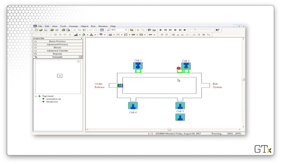
In this demo, we'll be looking at the manufacturing cell we just described. Here's our setup.
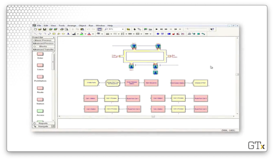
Let's take a look at the demo in action. We can see three different colors of marbles - red, green, and blue - which correspond to the three products that our cell can make. Each type of product traverses a different path through the system:
- Blue: one, two, three, four
- Red: one, two, four, two, three
- Green: two, one, three
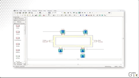
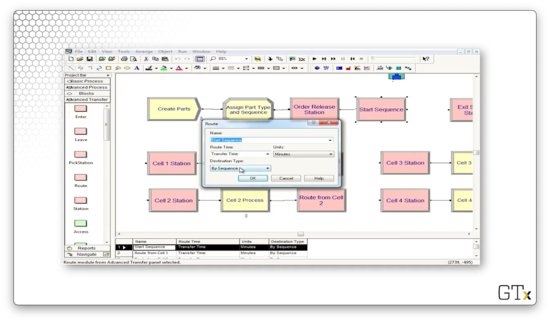
Let's look at the code. We create parts and then immediately assign them their part type and their sequence. From there, the part starts their sequence. For example, a blue part would immediately go to the "Cell 1 Station" block, the first in their sequence.
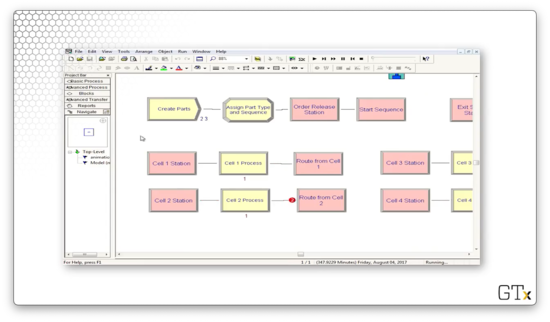
Let's look at the configuration for the Route block named "Start Sequence". This block has a Route Time of "Transfer Time", where "Transfer Time" is a variable that we created and set to "2". The Destination Type is determined "By Sequence". In short, it takes two minutes to route a part to the next station, as defined by its sequence.
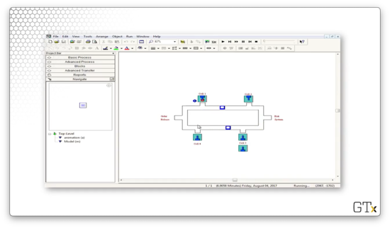
Now let's look at a demo involving machine movement. The small green square represents a transporter, which can shuttle parts from station to station.
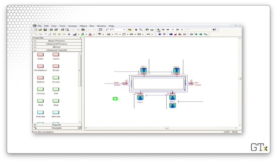
Here we see transporters in use, now in blue, navigating through the system to pick up new parts.
If we need more transporters, we can select the Transporter spreadsheet from the Advanced Transfer template and adjust the Number of Units field.
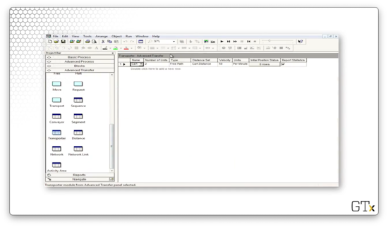
Now we can see that we have four transporters instead of two.
OMSCS Notes is made with in NYC by Matt Schlenker.
Copyright © 2019-2023. All rights reserved.
privacy policy