Simulation
Input Analysis
89 minute read
Notice a tyop typo? Please submit an issue or open a PR.
Input Analysis
Introduction
The goal of input analysis is to ensure that the random variables we use in our simulations adequately approximate the real-world phenomena we are modeling. We might use random variables to model interarrival times, service times, breakdown times, or maintenance times, among other things. These variables don't come out of thin air; we have to specify them appropriately.
Why Worry? GIGO!
If we specify our random variables improperly, we can end up with a GIGO simulation: garbage-in-garbage-out. This situation can ruin the entire model and invalidate any results we might obtain.
GIGO Example
Let's consider a single-server queueing system with constant service times of ten minutes. Let's incorrectly assume that we have constant interarrival times of twelve minutes. We should expect to never have a line under this assumption because the service times are always shorter than the interarrival times.
However, suppose that, in reality, we have Exp(12) interarrival times. In this case, the simulation never sees the line that actually occurs. In fact, the line might get quite long, and the simulation has no way of surfacing that fact.
So What To Do?
Here's the high-level game plan for performing input analysis. First, we'll collect some data for analysis for any random variable of interest. Next, we'll determine, or at least estimate, the underlying distribution along with associated parameters: for example, Nor(30,8). We will then conduct a formal statistical test to see if the distribution we chose is "approximately" correct. If we fail the test, then our guess is wrong, and we have to go back to the drawing board.
Identifying Distributions
In this lesson, we will look at some high-level methods for examining data and guessing the underlying distribution.
Three Little Bears
We can always present data in the form of a histogram. Suppose we collect one hundred observations, and we plot the following histogram. We can't really determine the underlying distribution because we don't have enough cells.

Suppose we plot the following histogram. The resolution on this plot is too granular. We can potentially see the underlying distribution, but we risk missing the forest for the trees.
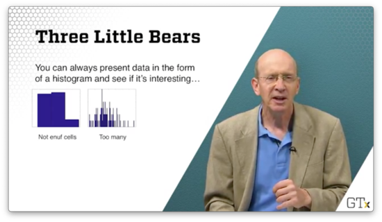
If we take the following histogram, we get a much clearer picture of the underlying distribution.
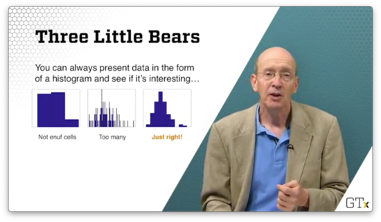
It turns out that, if we take enough observations, the histogram will eventually converge to the true pdf/pmf of the random variable we are trying to model, according to the Glivenko–Cantelli theorem.
Stem-and-Leaf
If we turn the histogram on its side and add some numerical information, we get a stem-and-leaf diagram, where each stem represents the common root shared among a collection of observations, and each leaf represents the observation itself.

Which Distribution?
When looking at empirical data, what questions might we ask to arrive at the underlying distribution? For example, can we at least tell if the observations are discrete or continuous?
We might want to ask whether the distribution is univariate or multivariate. We might be interested in someone's weight, but perhaps we need to generate height and weight observations simultaneously.
Additionally, we might need to check how much data we have available. Certain distributions lend themselves more easily to smaller samples of data.
Furthermore, we might need to communicate with experts regarding the nature of the data. For example, we might want to know if the arrival rate changes at our facility as the day progresses. While we might observe the rate directly, we might want to ask the floor supervisor what to expect beforehand.
Finally, what happens when we don't have much or any data? What if the system we want to model doesn't exist yet? How might we guess a good distribution?
Which Distribution, II?
Let's suppose we know that we have a discrete distribution. For example, we might realize that we only see a finite number of observations during our data collection process. How do we determine which discrete distribution to use?
If we want to model success and failures, we might use a Bernoulli random variable and estimate . If we want to look at the number of successes in trials, we need to consider using a binomial random variable.
Perhaps we want to understand how many trials we need until we get our first success. In that case, we need to look at a geometric random variable. Alternatively, if we want to know how many trials we need until the th success, we need a negative binomial random variable.
We can use the Poisson() distribution to count the number of arrivals over time, assuming that the arrival process satisfies certain elementary assumptions.
If we honestly don't have a good model for the discrete data, perhaps we can use an empirical or sample distribution.
Which Distribution, III?
What if the distribution is continuous?
We might consider the uniform distribution if all we know about the data is the minimum and maximum possible values. If we know the most likely value as well, we might use the triangular distribution.
If we are looking at interarrival times from a Poisson process, then we know we should be looking at the Exp() distribution. If the process is nonhomogeneous, we might have to do more work, but the exponential distribution is a good starting point.
We might consider the normal distribution if we are looking at heights, weights, or IQs. Furthermore, if we are looking at sample means or sums, the normal distribution is a good choice because of the central limit theorem.
We can use the Beta distribution, which generalizes the uniform distribution, to specify bounded data. We might use the gamma, Weibull, Gumbel, or lognormal distribution if we are dealing with reliability data.
When in doubt, we can use the empirical distribution, which is based solely on the sample.
Game Plan
As we said, we will choose a "reasonable" distribution, and then we'll perform a hypothesis test to make sure that our choice is not too ridiculous.
For example, suppose we hypothesize that some data is normal. This data should fall approximately on a straight line when we graph it on a normal probability plot, and it should look normal when we graph it on a standard plot. At the very least, it should also pass a goodness-of-fit test for normality, of which there are several.
Unbiased Point Estimation
It's not enough to decide that some sequence of observations is normal; we still have to estimate and . In the next few lessons, we will look at point estimation, which lets us understand how to estimate these unknown parameters. We'll cover the concept of unbiased estimation first.
Statistic Definition
A statistic is a function of the observations that is not explicitly dependent on any unknown parameters. For example, the sample mean, , and the sample variance, , are two statistics:
Statistics are random variables. In other words, if we take two different samples, we should expect to see two different values for a given statistic.
We usually use statistics to estimate some unknown parameter from the underlying probability distribution of the 's. For instance, we use the sample mean, , to estimate the true mean, , of the underlying distribution, which we won't normally know. If is the true mean, then we can take a bunch of samples and use to estimate . We know, via the law of large numbers that, as , .
Point Estimator
Let's suppose that we have a collection of iid random variables, . Let be a function that we can compute based only on the observations. Therefore, is a statistic. If we use to estimate some unknown parameter , then is known as a point estimator for .
For example, is usually a point estimator for the true mean, , and is often a point estimator for the true variance, .
should have specific properties:
- Its expected value should equal the parameter it's trying to estimate. This property is known as unbiasedness.
- It should have a low variance. It doesn't do us any good if is bouncing around depending on the sample we take.
Unbiasedness
We say that is unbiased for if . For example, suppose that random variables, are iid anything with mean . Then:
Since , is always unbiased for . That's why we call it the sample mean.
Similarly, suppose we have random variables, which are iid . Then, is unbiased for . Even though is unknown, we know that is a good estimator for .
Be careful, though. Just because is unbiased for does not mean that is unbiased for : . In fact, is biased for in this exponential case.
Here's another example. Suppose that random variables, are iid anything with mean and variance . Then:
Since , is always unbiased for . That's why we called it the sample variance.
For example, suppose random variables are iid . Then is unbiased for .
Let's give a proof for the unbiasedness of as an estimate for . First, let's convert into a better form:
Let's rearrange the middle sum:
Remember that represents the average of all the 's: . Thus, if we just sum the 's and don't divide by , we have a quantity equal to :
Now, back to action:
Let's take the expected value:
Note that is the same for all , so the sum is just :
We know that , so . Therefore:
Remember that , so:
Furthermore, remember that . Therefore:
Unfortunately, while is unbiased for the variance , is biased for the standard deviation .
Mean Squared Error
In this lesson, we'll look at mean squared error, a performance measure that evaluates an estimator by combining its bias and variance.
Bias and Variance
We want to choose an estimator with the following properties:
- Low bias (defined as the difference between the estimator's expected value and the true parameter value)
- Low variance
Furthermore, we want the estimator to have both of these properties simultaneously. If the estimator has low bias but high variance, then its estimates are meaninglessly noisy. Its average estimate is correct, but any individual estimate may be way off the mark. On the other hand, an estimator with low variance but high bias is very confident about the wrong answer.
Example
Suppose that we have random variables, . We know that our observations have a lower bound of , but we don't know the value of the upper bound, . As is often the case, we sample many observations from the distribution and use that sample to estimate the unknown parameter.
Consider two estimators for :
Let's look at the first estimator. We know that , by definition. Similarly, we know that , since is always unbiased for the mean. Recall how we compute the expected value for a uniform random variable:
Therefore:
As we can see, is unbiased for .
It's also the case that is unbiased, but it takes more work to demonstrate. As a first step, take the cdf of the maximum of the 's, . Here's what looks like:
If , and is the maximum, then is the probability that all the 's are less than . Since the 's are independent, we can take the product of the individual probabilities:
Now, we know, by definition, that the cdf is the integral of the pdf. Remember that the pdf for a uniform distribution, , is:
Let's rewrite :
Again, we know that the pdf is the derivative of the cdf, so:
With the pdf in hand, we can get the expected value of :
Note that , so is not an unbiased estimator for . However, remember how we defined :
Thus:
Therefore, is unbiased for .
Both indicators are unbiased, so which is better? Let's compare variances now. After similar algebra, we see:
Since the variance of involves dividing by , while the variance of only divides by , has a much lower variance than and is, therefore, the better indicator.
Bias and Mean Squared Error
The bias of an estimator, , is the difference between the estimator's expected value and the value of the parameter its trying to estimate: . When , then the bias is and the estimator is unbiased.
The mean squared error of an estimator, , the expected value of the squared deviation of the estimator from the parameter: .
Remember the equation for variance:
Using this equation, we can rewrite :
Usually, we use mean squared error to evaluate estimators. As a result, when selecting between multiple estimators, we might not choose the unbiased estimator, so long as that estimator's MSE is the lowest among the options.
Relative Efficiency
The relative efficiency of one estimator, , to another, , is the ratio of the mean squared errors: . If the relative efficiency is less than one, we want ; otherwise, we want .
Let's compute the relative efficiency of the two estimators we used in the previous example:
Remember that both estimators are unbiased, so the bias is zero by definition. As a result, the mean squared errors of the two estimators is determined solely by the variance:
Let's calculate the relative efficiency:
The relative efficiency is greater than one for all , so is the better estimator just about all the time.
Maximum Likelihood Estimation
In this lesson, we are going to talk about maximum likelihood estimation, which is perhaps the most important point estimation method. It's a very flexible technique that many software packages use to help estimate parameters from various distributions.
Likelihood Function and Maximum Likelihood Estimator
Consider an iid random sample, , where each has pdf/pmf . Additionally, suppose that is some unknown parameter from that we would like to estimate. We can define a likelihood function, as:
The maximum likelihood estimator (MLE) of is the value of that maximizes . The MLE is a function of the 's and is itself a random variable.
Exponential Example
Consider a random sample, . Find the MLE for . Note that, in this case, , is taking the place of the abstract parameter, . Now:
We know that exponential random variables have the following pdf:
Therefore:
Let's expand the product:
We can pull out a term:
Remember what happens to exponents when we multiply bases:
Let's apply this to our product (and we can swap in notation to make things easier to read):
Now, we need to maximize with respect to . We could take the derivative of , but we can use a trick! Since the natural log function is one-to-one, the that maximizes also maximizes . Let's take the natural log of :
Let's remember three different rules here:
Therefore:
Now, let's take the derivative:
Finally, we set the derivative equal to and solve for :
Thus, the maximum likelihood estimator for is , which makes a lot of sense. The mean of the exponential distribution is , and we usually estimate that mean by . Since is a good estimator for , it stands to reason that a good estimator for is .
Conventionally, we put a "hat" over the that maximizes the likelihood function to indicate that it is the MLE. Such notation looks like this: .
Note that we went from "little x's", , to "big x", , in the equation. We do this to indicate that is a random variable.
Just to be careful, we probably should have performed a second-derivative test on the function, , to ensure that we found a maximum likelihood estimator and not a minimum likelihood estimator.
Bernoulli Example
Let's look at a discrete example. Suppose we have . Let's find the MLE for . We might remember that the expected value of Bern() random variable is , so we shouldn't be surprised if is our MLE.
Let's remember the values that can take:
Therefore, we can write the pmf for a Bern() random variable as follows:
Now, let's calculate . First:
Remember that . So:
Let's take the natural log of both sides, remembering that :
Let's take the derivative, remembering that the derivative of equals :
Now we can set the derivative equal to zero, and solve for :
MLE Examples
In this lesson, we'll look at some additional MLE examples. MLEs will become very important when we eventually carry out goodness-of-fit tests.
Normal Example
Suppose we have . Let's find the simultaneous MLE's for and :
Let's take the natural log:
Let's take the first derivative with respect to , to find the MLE, , for . Remember that the derivative of terms that don't contain are zero:
What's the derivative of with respect to ? Naturally, it's . Therefore:
We can set the expression on the right equal to zero and solve for :
If we solve for , we see that , which we expect. In other words, the MLE for the true mean, , is the sample mean, .
Now, let's take the derivative of with respect to . Consider:
We can set the expression on the right equal to zero and solve for :
Notice how close is to the unbiased sample variance:
Because is unbiased, we have to expect that is slightly biased. However, has slightly less variance than , making it the MLE. Regardless, the two quantities converge as grows.
Gamma Example
Let's look at the Gamma distribution, parameterized by and . The pdf for this distribution is shown below. Recall that is the gamma function.
Suppose we have . Let's find the MLE's for and :
Let's take the natural logarithm of both sides, remembering that :
Let's get the MLE of first by taking the derivative with respect to . Notice that the middle two terms disappear:
Let's set the expression on the right equal to zero and solve for :
It turns out the mean of the Gamma distribution is . If we pretend that then we can see how, with a simple rearrangement, that .
Now let's find the MLE of . First, we take the derivative with respect to :
We can define the digamma function, , to help us with the term involving the gamma function and it's derivative:
At this point, we can substitute in , and then use a computer to solve the following equation, either by bisection, Newton's method, or some other method:
The challenging part of evaluating the digamma function is computing the derivative of the gamma function. We can use the definition of the derivative here to help us, choosing our favorite small and then evaluating:
Uniform Example
Suppose we have . Let's find the MLE for .
Remember that the pdf . We can take the likelihood function as the product of the 's:
In order to have , we must have . In other words, must be at least as large as the largest observation we've seen yet: .
Subject to this constraint, is not maximized at . Instead is maximized at the smallest possible value, namely .
This result makes sense in light of the similar (unbiased) estimator that we saw previously.
Invariance Properties of MLEs
In this lesson, we will expand the vocabulary of maximum likelihood estimators by looking at the invariance property of MLEs. In a nutshell, if we have the MLE for some parameter, then we can use the invariance property to determine the MLE for any reasonable function of that parameter.
Invariance Property of MLE's
If is the MLE of some parameter, , and is a 1:1 function, then is the MLE of .
Remember that this invariance property does not hold for unbiasedness. For instance, we said previously that the sample variance is an unbiased estimator for the true variance because . However, , so we cannot use the sample standard deviation as an unbiased estimator for the true standard deviation.
Examples
Suppose we have a random sample, . We might remember that the MLE of is . If we consider the 1:1 function , then the invariance property says that the MLE of is .
Suppose we have a random sample, . We saw previously that the MLE for is:
We just said that we couldn't take the square root of to estimate in an unbiased way. However, we can use the square root of to get the MLE for .
If we consider the 1:1 function , then the invariance property says that the MLE of is:
Suppose we have a random sample, . The survival function, , is:
We saw previously the the MLE for is .Therefore, using the invariance property, we can see that the MLE for is :
The MLE for the survival function is used all the time in actuarial sciences to determine - somewhat gruesomely, perhaps - the probability that people will live past a certain age.
The Method of Moments (Optional)
In this lesson, we'll finish off our discussion on estimators by talking about the Method of Moments.
The Method Of Moments
The th moment of a random variable is:
Suppose we have a sequence of random variables, , which are iid from pmf/pdf . The method of moments (MOM) estimator for , , is:
Note that is equal to the sample average of the 's. Indeed, the MOM estimator for , is the sample mean, :
Similarly, we can find the MOM estimator for :
We can combine the MOM estimators for to produce an expression for the variance of :
Of course, it's perfectly okay to use to estimate the variance, and the two quantities converge as grows.
Poisson Example
Suppose that . We know that, for the Poisson distribution, , so a MOM estimator for is .
We might remember that the variance of the Poisson distribution is also , so another MOM estimator for is:
As we can see, we have two different estimators for , both of which are MOM estimators. In practice, we usually will use the easier-looking estimator if we have a choice.
Normal Example
Suppose that . We know that the MOM estimators for and are and , respectively. For this example, these estimators happen to be the same as the MLEs.
Beta Example
Now let's look at a less trivial example. Here we might really rely on MOM estimators because we cannot find the MLEs so easily.
Suppose that . The beta distribution has the following pdf:
After much algebra, it turns out that:
Let's find MOM estimators for and . Given the expected value above, let's solve for :
Since we know that is the MOM estimator for , we have a reasonable approximation for :
We can solve for by making the following substitutions into the variance equation above: for , for , and the approximation of , in terms of and , for . After a bunch of algebra, we have the MOM estimator for :
Let's plug back into our approximation for to get in terms of and :
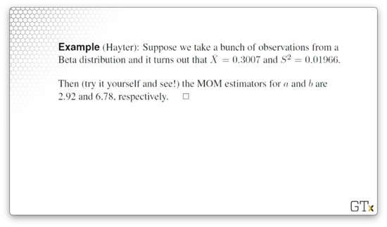
If we plug and chug with the following and , we should get the following values for the MOM estimators for and .
Goodness-of-Fit Tests
In this lesson, we'll start our discussion on goodness-of-fit tests. We use these tests to assess whether a particular simulation input distribution accurately reflects reality.
What We've Done So Far
Until now, we've guessed at reasonable distributions and estimated the relevant parameters based on the data. We've used different estimators, such as MLEs and MOM estimators. Now we will conduct a formal test to validate the work we've done. If our guesses and estimations are close, our tests should reflect that.
In particular, we will conduct a formal hypothesis test to determine whether a series of observations, , come from a particular distribution with pmf/pdf, . Here's our null hypothesis:
We will perform this hypothesis test at a level of significance, , where:
As usual, we assume that is true, only rejecting it if we get ample evidence to the contrary. The distribution is innocent until proven guilty. Usually, we choose to be or .
High-Level View of Goodness-Of-Fit Test Procedure
Let's first divide the domain of into sets, . If is discrete, then each set will consist of distinct points. If is continuous, then each set will contain an interval.
Second, we will tally the number of observations that fall into each set. We refer to this tally as . For example, refers to the number of observations we see in . Remember that , where is the total number of observations we collect.
If , then . In other words counts the number of sucesses - landing in set - given trials, where the probability of success is . Because is binomial, the expected number of observations that fall in each set, assuming is .
Next, we calculate a test statistic based on the differences between the 's and 's. The chi-squared g-o-f test statistic is:
If the distribution we've guessed fits the data well, then the 's and 's will be very close, and will be small. On the other hand, if we've made a bad guess, will be large.
As we said, a large value of indicates a bad fit. In particular, we reject if:
Remember that refers to the number of sets we have generated from the domain of , and refers to the level of significance at which we wish to conduct our test.
Here, refers to the number of unknown parameters from that have to be estimated. For example, if , then . If , then .
Additionally, refers to the quantile of the distribution. Specifically:
If , we fail to reject .
Remarks
In order to ensure that the test gives good results, we want to select such that and pick .
If the degrees of freedom, , is large, than we can approximate using the corresponding standard normal quantile, :
If we don't want to use the goodness-of-fit test, we can use a different test, such as Kolmogorov-Smirnov, Anderson-Darling, or Shapiro-Wilk, among others.
Uniform Example
Let's test our null hypothesis that a series of observations, , are iid Unif(0,1). Suppose we collect observations, where , and we divide the unit interval into sets. Consider the following 's and 's below:
The 's refer to the actual number of observations that landed in each interval. Remember that, since , .
Let's calculate our goodness-of-fit statistic:
Let's set our significance level to . Since there are no unknown parameters, , so . Therefore:
Since , we fail to reject the null hypothesis and begrudgingly accept that the 's are iid Unif(0,1).
Discrete Example
Let's hypothesize that the number of defects in a printed circuit board follows a Geometric() distribution. Let's look at a random sample of boards and observe the number of defects. Consider the following table:
Now let's test the null hypothesis that . We can start by estimating via the MLE. The likelihood function is:
Let's take the natural log of both sides:
Now, let's take the derivative:
Now, let's set the expression on the right to zero and solve for :
We know that, for , . Therefore, it makes sense that our estimator, , is equal to . Anyway, let's compute :
Given , let's turn to the goodness-of-fit test statistic. We have our 's, and now we can compute our 's. By the invariance property of MLEs, the MLE for the expected number of boards, , having a particular number of defects, , is equal to .
Consider the following table. Of course, can take values from to , so we'll condense into the last row of the table.
Remember that we said we'd like to ensure that in order for the goodness-of-fit test to work correctly. Unfortunately, in this case, . No problem. Let's just roll into :
Let's compute the test statistic:
Now, let's compare our test statistic to the appropriate quantile. We know that , since we partitioned the values that can take into four sets. We also know that , since we had to estimate one parameter. Given :
Since , we reject and conclude that the number of defects in circuit boards probably isn't geometric.
Exponential Example
In this lesson, we'll apply a goodness-of-fit test for the exponential distribution. It turns out that we can apply the general recipe we'll walk through here to other distributions as well.
Continuous Distributions
For continuous distributions, let's denote the intervals . For convenience, we want to choose the 's such that has an equal probability of landing in any interval, . In other words:
Example
Suppose that we're interested in fitting a distribution to a series of interarrival times. Let's assume that the observations are exponential:
We want to perform a goodness-of-fit test with equal-probability intervals, which means we must choose 's such that:
If the intervals are equal probability, then the probability that an observation falls in any of the intervals must equal . Correspondingly, must increase by as it sweeps through each interval, until .
In any event, let's solve for :
Unfortunately, is unknown, so we cannot calculate the 's. We have to estimate . Thankfully, we might remember that the MLE is . Thus, by the invariance property, the MLEs of the 's are:
Suppose that we take observations and divide them into equal-probability intervals. Let's also suppose that the same mean based on these observations is . Then:
Given this formula, let's compute our first equal-probability interval:
What's the expected number of observations in each interval? Well, since we made sure to create equal-probability intervals, the expected value for each interval is:
Now let's tally up how many observations fall in each interval, and record our 's. Consider the following table:
Given these observations and expectations, we can compute our goodness-of-fit statistic:
Let's choose the appropriate quantile. We'll use and . Since - remember, we estimated - then . Therefore:
Since our test statistic is greater than our quantile, we must reject and conclude that the observations are not exponential.
Weibull Example
In this lesson, we'll carry out a goodness-of-fit test for observations supposedly coming from the Weibull distribution. This procedure will take more work than the exponential, but it's more general, as the Weibull generalizes the exponential.
Weibull Example
Let's suppose that we have a series of observations, , and we hypothesize that they are coming from a Weibull(, ) distribution. The Weibull distribution has the following cdf:
We say that the Weibull generalizes the exponential because, for , is the cdf of the exponential distribution:
Like we did with the exponential, we'd like to conduct a goodness-of-fit test with equal-probability intervals. In other words, we will choose interval boundaries, 's, such that:
If the intervals are equal probability, then the probability that an observation falls in any of the intervals must equal . Correspondingly, must increase by as it sweeps through each interval, until .
Let's now solve for :
Since and are unknown, we'll have two MLEs, so . Remember that is a parameter whose value we subtract from the degrees of freedom of the distribution whose quantile we take during our test.
Let's differentiate the cdf, , to get the pdf, :
From there, we can take the likelihood function for an iid sample of size :
If we take the natural logarithm of the likelihood function, we get:
Now, we have to maximize with respect to and . To do so, we take the partial derivative of with respect to the appropriate parameter, set it to zero, and solve for that parameter. After a bunch of algebra, we get this value for :
Correspondingly, we get the following function for , such that :
How do we find the zero? Let's try Newton's method. Of course, to use this method, we need to know the derivative of :
Here's a reasonable implementation of Newton's method. Let's initialize , where is the sample mean, and is the sample variance. Then, we iteratively improve our guess for , using Newton's method:
If , then we stop and set the MLE . Otherwise, we continue refining . Once we have , to which Newton's method converges after only three or four iterations, we can immediately get :
Then, by invariance, we finally have the MLEs for the equal-probability interval endpoints:
Let's suppose we take observations and divide them into equal-probability intervals. Moreover, let's suppose that we calculate that and . Given these parameters:
Further suppose that we get the following 's:
Let's compute our goodness-of-fit statistic:
Given and , our quantile is:
Since our test statistic is less than our quantile, we fail to reject the null hypothesis and assume that the observations are coming from a Weibull distribution.
Still More Goodness-of-Fit Tests
In this lesson, we'll look at other types of goodness-of-fit tests. In particular, we will look at Kolmogorov-Smirnov, which works well when we have small samples.
Kolmogorov-Smirnov Goodness-of-Fit Test
There are plenty of goodness-of-fit tests that we can use instead of the test. The advantage of the Kolmogorov-Smirnov test (K-S) is that it works well in low-data situations, although we can use it perfectly well when we have ample data, too.
As usual, we'll test the following null hypothesis:
Recall that the empirical cdf, or sample cdf, of a series of observations, , is defined as:
In other words, the cdf of the sample, evaluated at , is equal to the ratio of observations less than or equal to to the total number of observations. Remember that is a step function that jumps by at each .
For example, consider the empirical cdf of ten Exp(1) observations - in blue below - on which we've superimposed the Exp(1) cdf, in red:
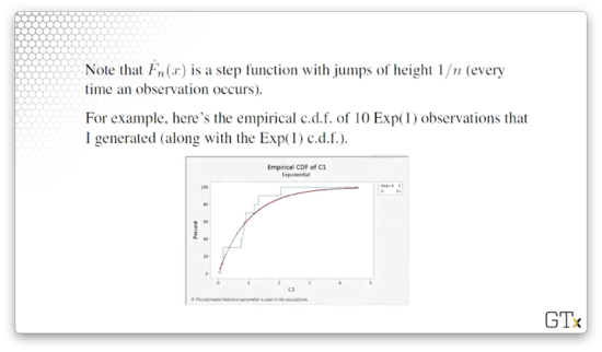
Notice that every time the empirical cdf encounters an observation, it jumps up by , or . If we look at the superimposed red line, we can see that the empirical cdf (generated from just ten observations) and the actual cdf fit each other quite well.
Indeed, the Glivenko-Cantelli Lemma says that the empirical cdf converges to the true cdf as the sample size increases: as . If is true, then the empirical cdf, , should be a good approximation to the true cdf, , for large .
We want to answer the main question: Does the empirical distribution actually support the assumption that is true? If the empirical distribution doesn't closely resemble the distribution that is supposing, we should reject .
In particular, the K-S test rejects if the following inequality holds:
In other words, we define our test statistic, , as the maximum deviation between the hypothesized cdf, , and the empirical cdf, . Note here that is our level of significance, and is a tabled K-S quantile. Interestingly, the value of depends on the particular distribution we are hypothesizing, in addition to and .
If the empirical cdf diverges significantly from the supposed true cdf, then will be large. In that case, we will likely reject the null hypothesis and conclude that the observations are probably not coming from the hypothesized cdf.
K-S Example
Let's test the following null hypothesis:
Of course, we've used the goodness-of-fit test previously to test uniformity. Also, we probably wouldn't test the uniformity of numbers coming from an RNG using K-S because, in that case, we'd likely have millions of observations, and a test would be just fine.
However, let's pretend that these 's are expensive to obtain, and therefore we only have a few of them; perhaps they are service times that we observed over the course of a day.
Remember the K-S statistic:
Now, remember the cdf for the uniform distribution:
For :
As a result, we can tighten the range of and substitute in the cdf. Consider:
The maximum can only occur when equals one of the observations, . At any , jumps suddenly from to . Since doesn't experience a jump itself at this point, the distance between and is maximized when equals some .
Let's first define the ordered points, . For example, if , , and , then , and .
Instead of computing the maximum over all the -values between zero and one, we only have to compute the maximum taken at the jump points. We can calculate the two potential maximum values:
Given those two values, it turns out that .
Let's look at a numerical example. Consider:
Let's calculate the and components:
As we can see from the bolded cells, , and , so . Now, we can go to a K-S table for the uniform distribution. We set and chose , and . Because the statistic is less than the quantile, we fail to reject uniformity.
That being said, we encountered several small numbers in our sample, leading us to perhaps intuitively feel as though these 's are not uniform. One of the properties of the K-S test is that it is quite conservative: it needs a lot of evidence to reject .
Other Tests
There are many other goodness-of-fit tests, such as:
- Anderson-Darling
- Cramér-von Mises
- Shapiro-Wilk (especially appropriate for testing normality)
We can also use graphical techniques, such as Q-Q plots, to evaluate normality. If observations don't fall on a line on a Q-Q plot, we have to question normality.
Problem Children
In this lesson, we will talk about performing input analysis under problematic circumstances.
Problem Children
We might think that we can always find a good distribution to fit our data. This assumption is not exactly true, and there are some situations where we have to be careful. For example, we might have little to no data or data that doesn't look like one of our usual distributions. We could also be working with nonstationary data; that is, data whose distribution changes over time. Finally, we might be dealing with multivariate or correlated data.
No / Little Data
Believe it or not, this issue turns up all the time. For example, at the beginning of every project, there simply are no observations available. Additionally, even if we have data, the data might not be useful when we receive it: it might contain unrealistic, or flat-out wrong, values, or it might not have been cleaned properly. As a concrete example, we can imagine receiving airport data that shows planes arriving before they depart.
What do we do in these situations? We can interview so-called "domain experts" and try to get at least the minimum, maximum, and "most likely" values from them so that we can guess at uniform or triangular distributions. If the experts can provide us with quantiles - what value we should expect 95% of the observations to fall below, for example - that's even better. At the very least, we can discuss the nature of the observations with the expert and try to extract some information that will allow us to make a good guess at the distribution.
If we have some idea about the nature of the random variables, perhaps we can start to make good guesses at the distribution. For example, if we know that the data is continuous, we know that a geometric distribution doesn't make sense. If we know that the observations have to do with arrival times, then we will treat them differently than if they are success/failure binaries.
Do the observations adhere to Poisson assumptions? If so, then we are looking at the Poisson distribution, if we are counting arrivals, or the exponential distribution, if we are working with interarrival times. Are the observations averages or sums? We might be able to use the central limit theorem and consider the normal distribution. If the observations are bounded, we might consider the beta distribution, which generalizes the uniform and triangular. We might consider the gamma, Weibull, or lognormal distributions if we are working with reliability data or job time data.
Perhaps we can understand something about the physical characteristics underlying the random variable. For example, the distribution of the particulate matter after an explosion falls in a lognormal distribution. We also might know that the price of a stock could follow the lognormal distribution.
Goofy Distributions
Let's consider a poorly designed exam with two modes: students either did quite well or very poorly. We can represent this distribution using some combination of two normal random variables, but most commercial software packages cannot fit distributions like this. For example, consider Minitab fitting a normal to the data below.
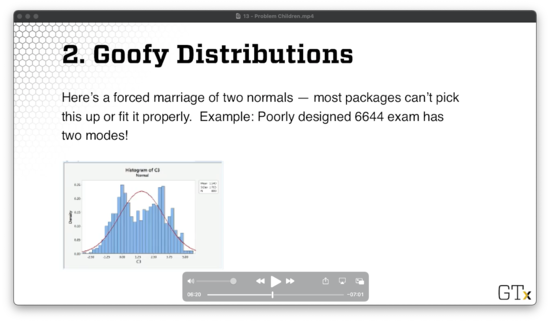
We can attempt to model such a distribution as a mixture of other reasonable distributions. Even easier, we can sample directly from the empirical distribution, or perhaps a smoothed version thereof, which is called bootstrapping.
Nonstationary Data
Arrival rates change over time. For example, consider restaurant occupancy, traffic on the highway, call center activity, and seasonal demand for products. We have to take this variability into account, or else we will get garbage-in-garbage-out.
One strategy we might use is to model the arrivals as a nonhomogeneous Poisson process, and we explored NHPPs back when we discussed random variate generation. Of course, we have to model the rate function properly. Arena uses a piecewise-constant rate function, which remains constant within an interval, but can jump up or down in between intervals.
Multivariate / Correlated Data
Of course, data don't have to be iid! Data is often multivariate. For example, a person's height and weight are correlated. When modeling people, we have to ensure that we generate the correlated height and weight simultaneously, lest we generate a seven-foot-tall person who weighs ninety pounds.
Data can also be serially correlated. For example, monthly unemployment rates are correlated: the unemployment rate next month is correlated with the rate this month (and likely the past several months). As another example, arrivals to a social media site might be correlated if something interesting gets posted, and the public hears about it. As a third example, a badly damaged part may require more service than usual at a series of stations, so the consecutive service times are likely correlated. Finally, if a server gets tired, his service times may be longer than usual.
What can we do? First, we need to identify situations in which data is multivariate or serially correlated, and we can conduct various statistical tests to surface these relationships. From there, we can propose appropriate models. For example, we can use the multivariate normal distribution if we are looking at heights and weights. We can also use time series models for serially correlated observations, such as the ARMA(p,q), EAR(1), and ARP processes we discussed previously.
Even if we guess at the model successfully, we still need to estimate the relevant parameters. For example, in the multivariate normal distribution, we have to estimate the marginal means and variances, as well as the covariances. Some parameters are easier to estimate than others. For a simple time series, like AR(1), we only have to estimate the coefficient, . For more complicated models, like ARMA(p,q) processes where p and q are greater than one, we have to use software, such as Box-Jenkins technology.
After we've guessed at the distribution and estimated that relevant parameters, we have to finally validate our estimated model to see if it is any good. If we run a simulation and see something that looks drastically different from the original process, we have to reevaluate.
Alternatively, we can bootstrap samples from an empirical distribution if we are fortunate enough to have a lot of data.
Demo Time
In this lesson, we will demonstrate how we carry out an elementary input analysis using Arena.
Software Interlude
Arena has functionality that automatically fits simple distributions to our data, which we can access from Tools > Input Analyzer. This input analyzer purportedly gives us the best distribution from its library, along with relevant sample and goodness-of-fit statistics.
ExpertFit is a specialty product that performs distribution fitting against a much larger library of distributions. Both Minitab and R have some distribution fitting functionality, but they are not as convenient as Arena and ExpertFit.
The only drawback to some of these programs is that they have issues dealing with the problem children we discussed previously.
Demo Time
Let's hop over to Arena. First, we click Tools > Input Analyzer. Next, we select File > New and then File > Data File > Use Existing... to get started. From there, we can select the relevant .dst file. Let's click on normal.dst and take a look at the data.
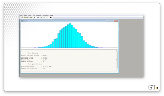
We can see that Arena gives us several pieces of information about our data, such as:
- number of observations (5000)
- minimum value (0.284)
- maximum value (7.29)
- sample mean (3.99)
- sample standard deviation (1)
We can try to fit various distributions by selecting from the Fit menu. Let's select Fit > Triangular and see what we get.
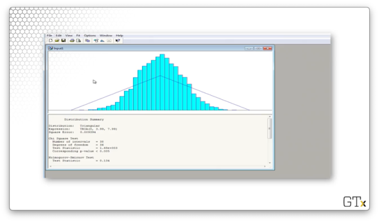
This distribution tries to fit the minimum, maximum, and modal values of the data, and, as we can see, it's a terrible fit. Arena believes that the best fit is a TRIA(0,3.99,7.99) distribution. The test statistic for this fit is 1680, and the corresponding p-value is less than 0.005. The K-S statistic is 0.134 and has a corresponding p-value of less than 0.01. In plain English, the data is not triangular.
Let's try again. We can select Fit > Weibull and see what we get.
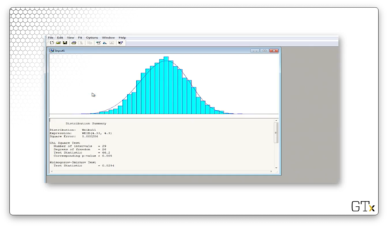
Arena believes that the best fit is a WEIB(4.33, 4.3) distribution. The test statistic for this fit is 66.2, and the corresponding p-value is less than 0.005. The K-S statistic is 0.0294 and has a corresponding p-value of less than 0.01. Again, even though the fit "looks" decent, we would still reject this data as being Weibull per the numbers.
Let's try again. We can select Fit > Erlang and see what we get.

Arena believes that the best fit is an ERLA(0.285, 14) distribution. The test statistic for this fit is 248, and the corresponding p-value is less than 0.005. The K-S statistic is 0.0414 and has a corresponding p-value of less than 0.01. The Erlang distribution does not fit this data.
Let's try again. We can select Fit > Normal and see what we get.

Arena believes that the best fit is a NORM(3.99, 1) distribution. The test statistic for this fit is 22.1, and the corresponding p-value is 0.732. The K-S statistic is 0.00789 and has a corresponding p-value greater than 0.15. We would fail to reject the null hypothesis in this case and conclude that this data is normal.
As a shortcut, we can select Fit > Fit All, and Arena will choose the best distribution from its entire library. If we select this option, Arena chooses the exact same normal distribution.
Let's look at some new data. We can click File > Data File > Use Existing... and then select the lognormal.dst file. Let's select Fit > Beta and see what we get.
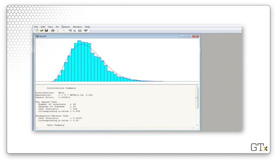
Arena believes that the best fit is a shifted, widened BETA(3.34, 8.82) distribution. The test statistic for this fit is 126, and the corresponding p-value is less than 0.005. The K-S statistic is 0.0239 and has a corresponding p-value of less than 0.01. The beta distribution is not a good fit.
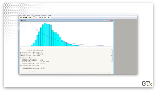
Let's try again. We can select Fit > Exponential and see what we get - what a joke.
Let's try again. We can select Fit > Weibull and see what we get.

Arena believes that the best fit is a shifted WEIB(2.49, 2.25) distribution. The test statistic for this fit is 237, and the corresponding p-value is less than 0.005. The K-S statistic is 0.0393 and has a corresponding p-value of less than 0.01. Clearly, Weibull is out.
Let's try again. We can select Fit > Lognormal and see what we get.

Arena believes that the best fit is a shifted LOGN(2.22, 1.14) distribution. The test statistic for this fit is 257, and the corresponding p-value is less than 0.005. The K-S statistic is 0.0458 and has a corresponding p-value of less than 0.01. Surprisingly, we would reject these observations as being lognormal, even though we know we sampled them from that distribution.
Let's select Fit > Fit All to see what Arena thinks is the best fit.

Arena believes that the best overall fit is a shifted ERLA(0.44, 5) distribution. The test statistic for this fit is 42.3, and the corresponding p-value is 0.0182. The K-S statistic is 0.0122 and has a corresponding p-value greater than 0.15. Depending on our significance level, we may reject or fail to reject this data as coming from the Erlang distribution.
Let's look at a final example. We can click File > Data File > Use Existing... and then select partbprp.dst file. Note that we don't know what distribution this data is coming from ahead of time.
Let's select Fit > Fit All to see what Arena thinks is the best fit.
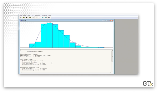
Arena believes that the best overall fit is a shifted GAMM(0.775, 4.29) distribution. The test statistic for this fit is 4.68, and the corresponding p-value is 0.337. The K-S statistic is 0.0727 and has a corresponding p-value greater than 0.15. We would fail to reject that this data is coming from the Gamma distribution.
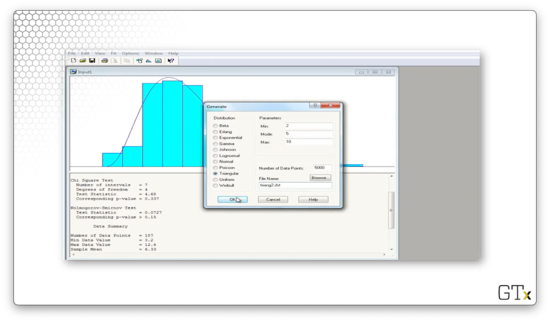
If we click on Data File > Generate New..., we can generate a file of observations according to some distribution. Let's write 5000 TRIA(2,5,10) observations to a file called triang2.dst.
Let's load these observations and then select Fit > Fit All.
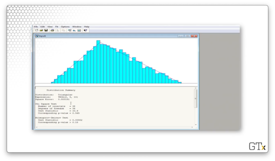
Arena believes that the best overall fit is a TRIA(2,5,10) distribution. The test statistic for this fit is 33.6, and the corresponding p-value is 0.565. The K-S statistic is 0.00932 and has a corresponding p-value greater than 0.15. Perfect.
OMSCS Notes is made with in NYC by Matt Schlenker.
Copyright © 2019-2023. All rights reserved.
privacy policy