Simulation
Course Tour
31 minute read
Notice a tyop typo? Please submit an issue or open a PR.
Course Tour
Whirlwind Tour
We are going to start our whirlwind tour of simulation by first talking about models. Then we will focus on defining and describing simulation, and, finally, we will think about how and when we might use simulation.
Models
Models are high-level representations of the operation of a real-world process or system. In this class, we will focus on models that are discrete, stochastic, and dynamic.
We can understand discrete models by understanding discrete systems. In a discrete system, things happen every once in a while. For example, in a queueing system, people arrive, people get served, and people leave. In between those events, nothing happens. Discrete models describe such discrete systems.
On the other hand, a continuous system is always changing. The weather is such a system, and we would refer to the corresponding models of the weather as continuous models.
Stochastic models concern probability and statistics. These models stand in contrast to deterministic models, which reflect basic cause and effect.
For example, a deterministic model might say that a customer definitively leaves after waiting in line for 5 minutes, while a stochastic model might say that a customer has a 50% chance of leaving.
Finally, dynamic models change over time, whereas static models stand still. For a static model, the same inputs produce the same outputs. In a dynamic model, a combination of the inputs plus some other state produces the outputs.
We can also consider different flavors of models from the perspective of how we might "solve" a model. Generally, there are three ways we might do this: analytical methods, numerical methods, and simulation.
Analytical methods are essentially simple equations. For example, we can model the relationship between the pressure and the volume of a gas using the ideal gas law. Analytical solutions are often only present for elementary systems.
If analytical methods don't work, we might turn to numerical methods. For example, the antiderivative of does not have a closed-form and therefore requires numerical integration methods.
If we can't use numerical methods, we have to resort to simulation. Simulation methods are much more general than analytical or numerical methods and can help us solve models that are much more complicated.
Examples of Models
We can toss a stone off a cliff and model that stone's position at different moments in time using simple physics equations. This is an example of an analytical model.
Modeling the weather is too complex for exact analytical methods, so we may have to turn to numerical methods. For example, we might have to solve a series of hundreds of thousands of partial differential equations. There are no closed-form solutions for models of this complexity.
If we add some randomness into the weather system, even the numerical methods might not work. We can make a simple system very difficult to model by injecting randomness in a specific way. At this point, we have to use simulation.
What is Simulation?
Simulation is the imitation of some real-world - or imaginary - process or system over time. Simulation involves first generating a history of the system being represented. We use that history to get data about the system and then draw inferences concerning how it operates.
Simulation is...
Simulation is one of the top three industrial engineering/operations research/management science technologies, along with statistics and engineering economics.
Simulation is an indispensable problem-solving methodology used successfully by academics and practitioners on a wide array of theoretical and applied problems.
What Is It Good For?
Simulation is an excellent tool for describing and analyzing the behavior of real and/or conceptual systems.
Simulation also allows us to explore and question system behavior. With simulation, we can ask "what if" questions, like what happens to queue waiting times if I add another server?
Simulation aids us in system design and optimization. For example, some aircraft companies will use simulation before they even consider building a new aircraft.
More broadly, we can simulate almost anything. For instance, we can simulate customer-based systems, like manufacturing systems, supply chains, and health systems. Additionally, we can simulate systems that don't have customers, such as stock and options pricing systems.
Reason to Simulate
We might use simulation to understand whether a system can accomplish its goals. For example, we may want a fast-food restaurant to complete orders within a particular time window. We can use simulation to determine if that goal is achievable, given the restaurant's current configuration.
If the current system is unable to accomplish its goals, simulation might help us identify which steps to take next. Sometimes simulation might point out a significant design flaw, while other times, it reveals that only a small tweak is necessary.
We can also use simulation to create a game plan. We can base different strategies on the outcomes of simulations of those different strategies to understand how to move forward. As a result, we can use simulations to resolve disputes about which approach is most effective.
We might use simulations to help sell our ideas. We can make simulations that are very visually appealing and easy to understand, and we can leverage this to help pitch our solutions.
Advantages
Simulation is advantageous for studying models that are far too complicated for analytical or numerical treatment. Additionally, simulation allows us to investigate detailed relations that those treatments might miss.
For instance, an analytical model might be able to report the exact expected waiting time in the queue. However, it won't necessarily reveal the percentage of customers having to wait a certain amount of time or what percentage of customers may leave the queue. A simulation can give you much more than just an "answer".
We can also use simulations as the basis for experimental studies of systems. We can simulate an experiment to understand how many trials we should run with the real data. On the flip side, we can use simulation to verify experimental results obtained through other methods.
Simulation ahead of implementation can help eliminate costly and embarrassing design blunders.
Disadvantages
While simulation can occasionally be easy, it often involves a lot of work. Simulation can require significant programming effort, and the data collection process required for effective simulation can be time-consuming and costly.
A more subtle disadvantage is that simulations do not give us an "answer"; instead, they typically provide random output. We need to interpret and communicate this randomness appropriately. For example, we might say that we expect a person to wait in a queue for 5 minutes, plus or minus 30 seconds.
Simulation is a great problem-solving technique, but, for specific problems, better methods exist. For example, if we are tossing a stone off a cliff - under ideal conditions - then simple physics equations are a sufficient model of behavior. Simulation is not a panacea!
History of Simulation
Simulation has been around a very long time - we will see an example shortly from several hundred years ago - but its use has exploded in the last fifty or sixty years alongside the rise of computers.
History
One of the first examples of simulation takes place in 1777 with Comte de Buffon. Buffon drew two parallel lines on the ground and then dropped many needles on the ground. He counted the number of times that a needle intersected one of the lines. From this simulation, known as Buffon's needle problem, Buffon was able to estimate .
Let's fast forward to the early 1900s. William Gosset was a statistician at the Guinness brewery in Ireland. In one simulation experiment, Gosset placed a bunch of samples of data - British prisoners' finger lengths, of all things - into a hat and withdrew them at random.
Guinness did not want to reveal that they hand a statistician on employ, so Gosset had to announce the results of this experiment using a pseudonym: Student. His simulation work gave rise to the Student's t-distribution.
More History
The first use of computer simulation occurred after World War II. Stan Ulam and John Von Neumann used simulation in the context of the development of the H-bomb; specifically, they simulated thermonuclear chain reactions. Indeed, the desire to model such reactions was a primary driver in creating the first computers.
Later, the 1950s and 1960s brought many industrial applications of simulation, namely, manufacturing problems and certain queueing models.
Recent History
Alongside these fledgling applications, people began to develop simulation languages. These languages meant that practitioners of simulation didn't have to reinvent the wheel every time they wanted to simulate a system.
Harry Markowitz, who won a Nobel Prize for his work on optimizing financial portfolios, was one of the first individuals to develop a simulation language, known as SIMSCRIPT.
After the 1960s, people began to put forth rigorous theoretical work related to simulation, such as the development of precise and efficient computation algorithms and probabilistic and statistical methods to analyze simulation output and input.
Origins: Manufacturing
For our purposes, simulation begins with manufacturing problems. Simulation became the technique of choice for this domain because many manufacturing problems had become too difficult to solve analytically or numerically.
For example, we might use simulation to understand the movement of parts through a system and the interactions between parts and system components like machines and other types of servers.
We can use simulation to examine conflicting demands for resources. If we have millions of parts flying through the system, and each part requires work from a particular machine or human, conflicts will arise. Simulation can help to reveal those conflicts.
Once we find conflicts, we can discuss different strategies for resolution. We can again employ simulation to try out different solutions before making changes to the real system.
We can also use simulation before even a first implementation of a system, which may help us see and avoid costly design blunders ahead of time.
Typical Questions
We might be curious about the throughput of a system. How many parts can we push through? We can generalize this idea of system performance out of manufacturing and consider it in different contexts. For example, we might be concerned with how many patients we can move through an emergency room.
Once we have a value for throughput, we might consider how we can change the throughput or change the system without changing the throughput. In one case, we might discover that we can add more servers to increase throughput. In another scenario, we might find that removing servers does not diminish throughput.
Particularly in manufacturing systems, we often encounter bottlenecks. Simulation helps us uncover bottlenecks. Furthermore, if we simulate how the system operates after removing specific bottlenecks, we might find different bottlenecks.
Suppose that we have to decide among several different designs for a system. We can use simulation to figure out which design will meet which criteria.
If we are looking at a giant network, we might want to make confident assertions about its reliability. Simulation can help us understand how to structure a network such that items move through it reliably.
Finally, we may want to understand what happens when a system breaks down. Should we have redundancy? At which layers? How long will it take to get the system back up to speed?
What Can We Do For You
We are going to talk about the kinds of problems we can solve using simulation. The punchline is that we can use simulation for just about anything: if we can describe it, we can simulate it.
What I Used to Think Simulation Was
Actual Applications
Simulation doesn't have to be just theoretical equations. We can apply simulation to real-life problems. In manufacturing, folks have done simulations of many different types of production facilities like automobile plants and carpet factories.
We can also use simulation for queueing problems. One of the canonical problems in this domain involves call center analysis. Simulation helps us understand how many servers a call center needs for calls to proceed in a timely fashion.
Another classic example here is modeling a fast-food drive-through. There is a particular restaurant near Georgia Tech where the drive-through line can only be about four or five cars before it starts extending into a busy street. Naturally, this restaurant is paranoid about keeping the line short.
We can simulate different strategies for moving customers through that line. For example, we could simulate a scenario in which employees take orders manually from the cars instead of waiting for people to reach the machine.
We can also simulate a fast-food call center! Let's suppose a large fast-food chain with many restaurants around the country wants to handle all orders through one central location. In other words, the person taking your order isn't located in the store. We can use simulation to understand how many restaurants we need before this type of centralization makes sense.
As a third example, folks have used simulation to understand and improve wait times in airport security lines.
Generic Supply Chain
Let's look at a generic supply chain, such as the one illustrated below.
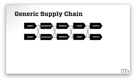
We can think about supply chains as giant queueing networks in which some nodes have to wait for other nodes. For example, the manufacturer has to wait for the supplier, the retailer must wait for the distributor, and the customer has to wait for everyone.
Supply Chains Continued
In the past, folks were not interested in simulating supply chains. When people spoke about supply chains, they spoke of averages, not probabilities.
For example, we might say that "on average," getting from point A to point B in the supply chain takes a certain amount of time.
However, averages aren't always the best metric for describing a system, because they don't take variability into account. Indeed, the flaw of averages explains how relying too heavily on averages can be problematic.
This ability to account for variation makes simulation such a valuable tool, and, today, supply-chain software often comes with simulation capabilities.
For example, we can use simulation to determine how much value a particular forecasting application provides in the supply chain. Additionally, we can use simulation to analyze randomness in the supply chain and model errors. These analyses help us understand if we have the best solution and, if not, what steps we might take to find it.
More Applications
Here are some of the domains in which we can use simulation:
- inventory and supply chain analysis
-
financial analysis
- portfolio analysis
- options pricing
- service sector
- health systems
We can use simulation to understand traffic flow and improve traffic engineering. For example, folks have uncovered, using simulation, scenarios in which adding a new lane increases traffic, somewhat counterintuitively.
Airspace simulation is related to traffic simulation. We might be curious to understand the time it takes for an airplane to get from one airport to another. Many different factors can influence this estimation. For example, a thunderstorm in Atlanta might delay flights destined for Hartsfield-Jackson airport.
Health Systems
There are many different opportunities for simulation in health systems. One classic example involves modeling patient flow in a hospital, which can help administrators understand throughput and wait times.
Optimizing doctor and nurse scheduling is a similar problem. A hospital can never know precisely how many people might show up in the emergency room on Friday night. If they haven't done proper scheduling, they could find themselves woefully understaffed in the face of a large influx of patients.
We can use simulation to understand how many rooms we might allocate for different purposes in the hospital. We might also use simulation to guide appropriate and sufficient procurement of supplies and inventory.
We might look at an individual patient and use simulation to understand if a particular disease is in the process of occurring. Relatedly, we might look at a population of individuals and simulate how a disease may spread amongst them. The characteristics of spread can change for diseases with different levels of virulence.
Georgia Tech does a lot of work with simulation around humanitarian logistics.
Surveillance Applications
We can use simulation to monitor time-series data; this is the essence of surveillance applications. We want to understand how and why data is changing over time. The main idea with surveillance is to predict issues as or before they happen. For example, is an influenza outbreak starting to occur now? Will the unemployment rate spike next quarter?
There is no shortage of examples of large companies being able to predict certain things with frightening accuracy. For example, Google might look at a customer's recent purchases and predict that they are pregnant, perhaps before they even know. For better or worse, we can now leverage massive data sets to generate better simulations than ever before.
Who's Mr. Handsome?

Dr. Harold Shipman
Dr. Harold Shipman - Mr. Handsome above - was a serial killer who used morphine and heroin overdoses to kill many of his patients, mostly older women.
He was caught after he carelessly revised a patient's will and left all of her assets to himself. Unfortunately for him, he used his typewriter to make the edits, which authorities were able to trace back to him.
As it turns out, he doctored the records to show that the patients had needed morphine, but the software recorded the dates of the transactions, and authorities were able to see the back-dated edits.
He never confessed to his crimes, and he hung himself in prison.
Simulation Can Help!
Sequential statistical hypothesis tests drive surveillance applications. These tests center around a null hypothesis, typically designated . We assume that is true - Dr. Shipman did not kill his patients - and then we gather evidence and see if we can disprove .
As an example of such hypothesis testing in society, we say that people are innocent until proven guilty. We start with a hypothesis that a person is innocent, and we assume that this hypothesis is true until enough evidence is present to refute it.
For complicated problems, the test statistics one might use to determine whether or not to reject the null hypothesis can have very complicated statistical distributions. These distributions are not likely to be normal or exponential or any other distribution that one learns about in an introductory statistics class.
We can use simulation to approximate the probability distributions of such test statistics. Then, when we take our sample data and compare it to the approximated distribution, we can reject if the sample casts doubt on the distribution.
This type of simulation work helped to reject the hypothesis that Dr. Shipman was not killing his patients. There was just too much evidence to the contrary.
Some Baby Examples
In this lesson, we will look at specific examples of the use of simulation in simple settings.
Happy Birthday
Let's first talk about the birthday paradox.
Assume that there are 365 days in a year - sorry, leap year babies - and that everybody has an equal chance of being born on any particular day, .
How many people do you need to have in a room to have at least a 50% chance that at least two people have the same birthday? Here are the choices:
- 9
- 23
- 42
- 183
Upon first hearing this problem, one might think that 183 is a reasonable choice. There are 365 possible birthdays, and 183 is roughly half that. As it turns out, with 183 people in the room, there is a greater than 99% chance that at least two of them share a birthday.
The reason for this counterintuitively high probability is that there are so many ways that 183 people can pair off. Remember, we are not just considering the probability that we share a birthday with any of the other 182 people, but also the probability that any of them shares a birthday with anyone else.
If we have 42 people in the room, our chances only drop to around 90%. As it turns out, we only need 23 people in the room to have just over a 50% chance that two of them share a birthday.
Simulating this problem is straightforward. We can begin sampling birthdays, each with probability , and count how many birthdays we have to sample before we get a match.
Here is a demonstration of such a simulation. In this particular example, we get a match after 19 randomly-sampled birthdays.
Each time we run the simulation, we sample different birthdays, and we might have to sample a different number of birthdays before we get a match. However, if we were to run infinite simulations, we would see that, on average, 50% of the simulations would draw the same birthday twice by the 23rd sample.
Notice in the demonstration above that we seed the simulation with the number 12345. While simulations appear to be random, they are not; in fact, the "randomness" is generated deterministically and is derived from this initial seed value. As a result, when we run the simulation using the same seed value, we select the same birthdays in the same order.
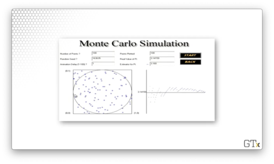
Let's Make Some Pi
Now we are going to use simulation to estimate .
Let's take a square and inscribe a circle inside it. If the circle has a radius, , then the circle has an area of , and the square has an area of (remember the side-length of the square is ).
We are going to start tossing darts at the square, and we can assume that we are equally likely to hit any point within the bounds of the square. As a result, the probability that a dart lands inside the inscribed circle is equal to the ratio of the circle's area to the square's: .
If we throw a massive number of darts, the proportion of the darts that land in the circle should approach , via the law of large numbers. If we multiply that proportion by four, we can get an estimate for : .
Bonus Quiz: What is the volume of a pizza with radius, , and height, ? Of course, it is , or pizza.
Let's run a simulation and see if we can approximate . In the images below, the simulated dart throws are on the left, and the corresponding running estimate of is on the right.
Here is the result of throwing 100 darts. Our estimate for after this simulation is 3.160.
Here is the result of throwing 1000 darts. Our estimate for after this simulation is 3.140.
Here is the result of throwing 100000 darts. Our estimate for after this simulation is 3.137.
Note that this estimation is slightly worse than the estimation from our simulation with 1000 darts. Simulations involve randomness, and randomness produces random error.
NB: I recreated this simulation for the web. Check it out here!
Fun With Calculus
In this example, we are going to use simulation to integrate the function from 0 to 1. Of course, we could compute this integral directly:
However, we are going to use simulation to approximate the integral using a pre-calculus methodology: rectangles. With this technique, we draw rectangles of width , where each rectangle is centered about a point, , along the x-axis and has a height of .
The idea here is that, as approaches , the sum of the triangles' areas approaches the integral of .
To approximate the integral via simulation, we are going to follow this same strategy. We sample points randomly from , and, for each point, , we construct a rectangle, centered about , with width and height .
Let's see if the sum of the rectangles' areas approaches the actual value of the integral as we increase .
With rectangles, the simulation produces an estimate of 0.5790.
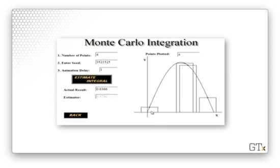
With rectangles, the simulation produces a better estimate: 0.6694.
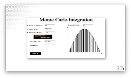
Finally, with rectangles, the estimate improves further to 0.6374.
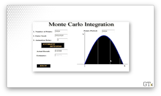
This type of simulated integration - Monte Carlo integration, specifically - is an elegant methodology to use in several applications that we will talk about in the course.
More Baby Examples
Let's look at some more baby examples.
Evil Random Numbers
Let's look at what happens when we use a "bad" random number generator (RNG). So far, we have talked about how RNGs are not truly random, but only appear to produce a sequence of random numbers. However, some RNGs do not even come close to generating random numbers. Unfortunately, such RNGs have been used in applications.
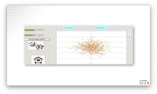
In this example, we are going to sample people's heights and weights from two normal distributions. We will assume that heights and weights are not correlated (a bad assumption, but not relevant to the demonstration).
Let's look at a plot of one such sampling process, where the origin represents the mean of both distributions, and each blue dot is a height/weight observation.
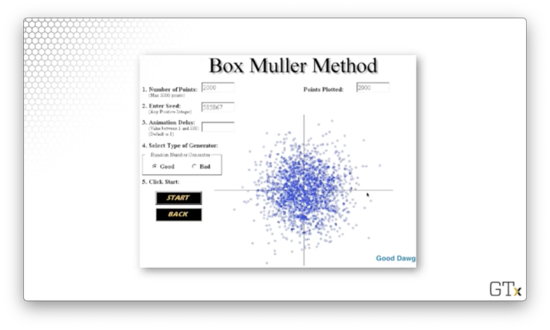
We can see several outliers; for example, there are some very tall, very heavy folks and some very short, very light folks. However, most of the observations occur close to the origin - the means - as we would expect when sampling from a normal distribution.
Let's generate 100 observations using a "good" RNG.
Let's try 1000 observations.
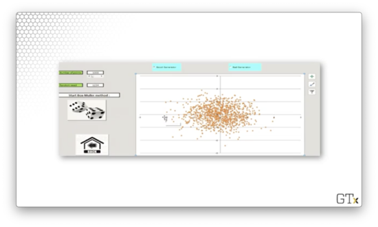
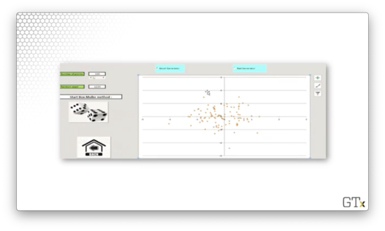
Both of these samples appear random. Now let's generate 1000 observations using a "bad" RNG.
Admittedly, this sample also looks random. So what's the issue? An RNG must work well for any possible seed value. For the "bad" RNG, seeds that are powers of two produce very non-random results. Let's see what sample is generated when the seed is 1024.
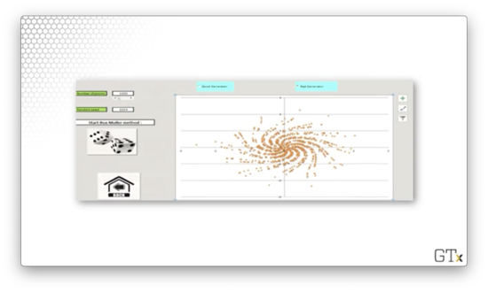
Beautiful, but definitely not random.
Queues 'R Us
Now we will take a look at a queueing problem.
Suppose we go to McWendy's, a popular burger joint, and we encounter a single-server queue: there is one line, with one server, and people get served first-in-first-out.
What happens as the arrival rate approaches the service rate?
- Nothing much
- The line gets pretty long
- Hamburgers start to taste better
We can use simulation to analyze the queuing model and answer this question.
One parameter that we need to specify for this type of simulation is the interarrival mean. This value describes how often a new customer shows up on average. Another parameter we need to specify is the service mean, which describes how long it takes for a customer to be served on average.
We refer to this type of queue as an MM1 queue. The two "M"'s stand for "Markovian/memoryless" and indicate that we are sampling both the interarrival times and service times from an exponential distribution. The "1" indicates that we are modeling a single-server queue. For more on this notation, see Kendall's notation.
Let's look at the results of an MM1 queue simulation.
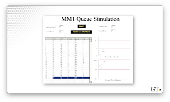
For this demonstration, we specified an interarrival mean of 4 and a service mean of 3, which means that customers tend to get served more quickly than they arrive. We could refer to this system as moderately congested.
In the tabular view on the bottom-left, we can see several rows, where each row describes a customer interacting with the system. For each customer, we have data points indicating when they arrived, how long it took them to be served, when they left and how long they waited.
The first customer arrives at time . Since the server is free, the customer is served immediately; he doesn't have to wait. Servicing this customer takes 7 minutes - not impossible when sampling from a distribution with a mean of three - and the customer leaves at time .
The second customer arrives at time . Unfortunately, there is someone ahead of him in the queue. As a result, he isn't served until that customer leaves: at time . After waiting for 5 minutes, the customer reaches the front of the queue and receives service after an additional 3 minutes, leaving at time .
Customer three arrives at time . At this point, customer one hasn't even left yet, and customer two has yet to be served. Customer two leaves the system at time , which is when customer three reaches the front of the queue. Having waited 5 minutes, he receives service after an additional 5 minutes, and he leaves at time .
The top graph in the bottom-right of the image above shows the queue length as a function of time, and the graph below it depicts server utilization as a function of time.
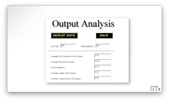
We can also generate summary statistics for this type of simulation.
Stock Market Follies
In this example, we will simulate a small portfolio of various stocks over five years. Each stock has an expected performance and an associated measure of volatility.
Let's look at our portfolio.
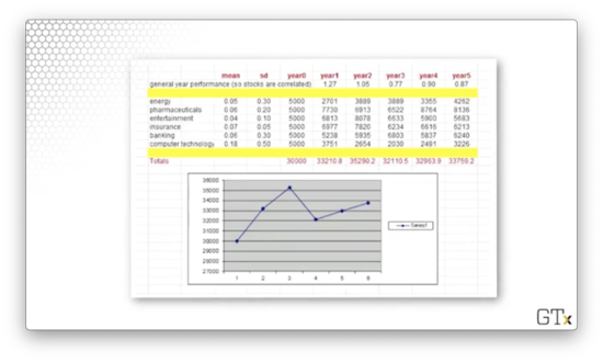
We hold stocks across six different sectors: energy, pharmaceuticals, entertainment, insurance, banking, and computer technology. Each stock's performance is parameterized by a mean, indicating average return, and a standard deviation, indicating volatility.
When we look at the means, it seems as though our portfolio can't decrease in value. However, a look at the standard deviations is sobering: the relatively modest expected gains are dwarfed by massive volatility.
For example, energy has a mean of 0.05 and a standard deviation of 0.3. As a result, 68% of samples from a distribution characterized by these statistics will fall between -0.25 and 0.35. There is plenty of room for bad performance in that spread.
We will start with $5,000 allocated to each stock, for a total portfolio value of $30,000. Then, we will simulate each stock's performance over the five years and aggregate them into a final portfolio value.
Let's try a simulation.
In this round, we did pretty well; after five years, we turned $30000 into more than $41000.
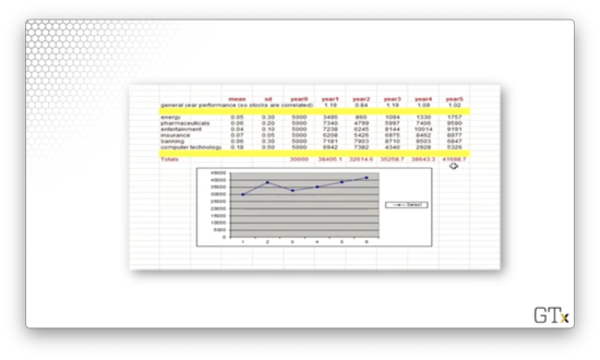
Let's try again.
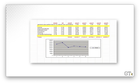
In this round, we did poorly. We lost almost $8000.
Let's try one more.
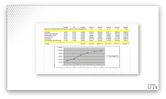
In this round, we were quite lucky. All of our stocks posted significant gains, and we ended up with almost $100,000 in our portfolio.
How do we make sense of such round-to-round variability? We can simulate our portfolio's performance, say, 1000 times and then compute summary statistics over the collection of final portfolio values.
Talk a Random Walk
Let's imagine that we are drunk. Every second we are going to take some steps to the left or the right. We can assume that the amount of space we move left or right is normally distributed. Where are we after seconds?
As increases, this "random walk" converges to something called Brownian motion. Albert Einstein, as well as Myron Scholes (of Black-Scholes model fame), won Nobel Prizes for their research on Brownian motion.
Look at the following image of Brownian motion.
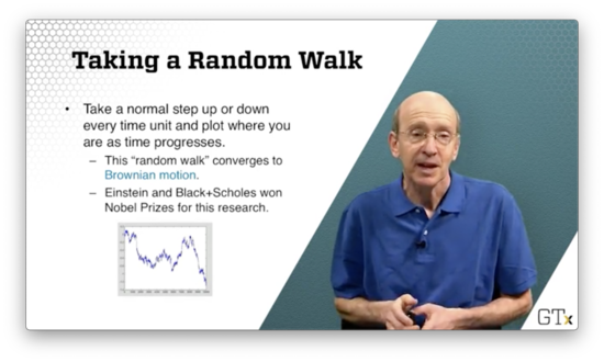
Doesn't that look like a plot of stock prices?
Generating Randomness
In this lesson, we are going to look at how we generate randomness. A spoiler alert: the algorithms that generate randomness are not random at all, but only appear random!
Randomness
Why do we care about randomness? Well, we need random variables (RVs) to run a simulation. For example, in our queueing simulation, we need interarrival times and service times.
The primary method we use to create randomness is to generate pseudo-random numbers (PRNs) from the uniform distribution, , using deterministic algorithms.
From there, we can apply transformations to these uniform random variables to produce new variables that come from different distributions: exponential distributions for interarrival times, normal distributions for heights, and so on.
Unif(0,1) PRNs
As we said, we use deterministic algorithms to generate these PRNs. One class of such algorithms is the linear congruential generators. Here is how they work.
We start with an integer seed value, , and we generate the next value in the sequence according to the following formula:
Remember that "mod" refers to the modulus function, which, for positive integers, is essentially the remainder function. For example, , as seven divided by four equals one with three remaining.
In creating these generators, we have to choose and carefully. Often, is a massive, prime number, and is a large number as well.
Notice that these generators produce integer values. To normalize these values - that is, compress them into the range - we divide them by . In other words:
Let's look at an example. Suppose that and our generator function is:
Let's calculate a few values in this sequence.
We can normalize these values by dividing by .
This generator is bad. The values that we get are clearly not uniformly distributed; indeed, it is impossible to produce a value outside of the set .
Here is a better generator:
This generator has specific properties that make it robust, including long "cycle times": the sequences does not repeat frequently. While this generator was used in several simulation languages for quite some time, better generators do exist.
Generating Other RVs
The PRNs that we generate are random variables drawn from the uniform distribution bounded by zero to one: .
Often, we'd like to generate random variables that come from other, more exciting distributions. We can apply the appropriate transformation to change the underlying distribution from which is sampled.
For example, we can apply the following transform to convert from a uniform random variable to an exponential random variable, using the inverse transform method:
There are more sophisticated methods available, such as the Box-Muller method for generating normally distributed random variables, and we will explore other such techniques as the course proceeds.
Simulation Output Analysis (OPTIONAL)
In this lesson, we are going to talk about simulation output. Random input means random output, and random output requires careful analysis. Simulation output is never independent or normal, so we need new methods for interpreting this output.
Analyzing Randomness
Let's consider the output of a simulation of customer waiting times at McWendy's.
The waiting times for consecutive customers are not normally distributed. Of course, waiting times can never be negative. Most people wait a certain amount of time, but there is often a large right tail; these skewed distributions are certainly not symmetrical, and therefore, not normal.
Also, the waiting times are not identically distributed because consumer behavior is different throughout the day. For example, there will likely be long lines of people at McWendy's during regular meal times - breakfast, lunch, and dinner. In between those times, however, customer arrival patterns are entirely different. Waiting times might frequently be zero during the slow parts of the day.
Finally, waiting times are not independent of each other. If we are waiting for a long time, then the poor guy next to us is also likely waiting for a long time. Our waiting time is correlated with his.
In summary, waiting times are not i.i.d. normal random variables. As a result, we cannot analyze this simulation output data using classical statistical methods.
Generally, there are two types of simulations that we are going to cover, and each requires a different approach regarding output analysis.
A terminating simulation gives us information about short-term behavior. We might use this type of simulation to understand waiting times in a bank over the course of a day or to simulate the average number of people infected during a (short-lived) pandemic. To analyze such simulations, we will use the method of independent replications.
A steady-state simulation gives us information about behavior over a much longer horizon. We might use this type of simulation to understand how a 24/7 assembly line operates over the course of a year. For analyzing these types of simulations, we can use the method of batch means, among other techniques.
Terminating Simulations
The method of independent replications involves running a simulation many times, each under identical conditions, and then applying classical statistics on the resulting collection of data points.
For example, we might simulate a queueing model one million times and then look at the mean and standard deviation of the collection of average wait times.
This conventional statistical treatment only works because we assume that the sample means from each run are approximately i.i.d. As it turns out, there is a lot of truth to this assumption.
Steady-State Simulations
In steady-state simulations, we first have to deal with initialization bias. In other words, we have to account for the fact that the state of the system at the beginning of the simulation is not indicative of the steady state.
For example, when we open a store for the day, there are no lines, and no one has to wait. However, if we examine the store at any time after that, we are likely to find folks waiting in line.
Usually, people "warm up" the simulation before collecting data. In our example, we might simulate the store for an hour before recording any observations. Failure to remove this initialization bias can ruin subsequent statistical analyses.
There are many different methods for dealing with steady-state data, which we will learn more about in due time:
- batch means
- overlapping batch means / spectral analysis
- standardized time series
- regeneration
The method of batch means involves slicing a long-running simulation - excluding the initial observations from the "warm up" - into contiguous, adjacent batches. We calculate the sample mean from each batch, again assuming that these values are approximately i.i.d. With this assumption in hand, we can again analyze the means using classical statistical techniques.
OMSCS Notes is made with in NYC by Matt Schlenker.
Copyright © 2019-2023. All rights reserved.
privacy policy