Happy studying! Did you find my notes useful this semester?
Please consider
giving me a few bucks
or
buying me a beer. Contributions like yours help me keep these notes forever free.
Happy studying! Did you find my notes useful this semester?
Please consider
giving me a few bucks
or
buying me a beer. Contributions like yours help me keep these notes forever free.
Calculus, Probability, and Statistics Primers, Continued
88 minute read
Notice a tyop typo? Please submit an
issue
or open a
PR.
Calculus, Probability, and Statistics Primers, Continued
Conditional Expectation (OPTIONAL)
In this lesson, we are going to continue our exploration of conditional expectation and look at several cool applications. This lesson will likely be the toughest one for the foreseeable future, but don't panic!
Conditional Expectation Recap
Let's revisit the conditional expectation of Y given X=x. The definition of this expectation is as follows:
For example, suppose f(x,y)21x2y/4 for x2≤y≤1. Then, by definition:
f(y∣x)=fX(x)f(x,y)
We calculated the marginal pdf, fX(x), previously, as the integral of f(x,y) over all possible values of y∈[x2,1]. We can plug in fX(x) and f(x,y) below:
f(y∣x)=821(1−x4)421x2y=1−x42y,x2≤y≤1
Given f(y∣x), we can now compute E[Y∣X=x]:
E[Y∣X=x]=∫Ry∗(1−x42y)dy
We adjust the limits of integration to match the limits of y:
E[Y∣X=x]=∫x21y∗(1−x42y)dy
Now, complete the integration:
E[Y∣X=x]=∫x211−x42y2dy
E[Y∣X=x]=1−x42∫x21y2dy
E[Y∣X=x]=1−x423y3∣∣∣∣x21
E[Y∣X=x]=3(1−x4)2y3∣∣∣∣x21=3(1−x4)2(1−x6)
Double Expectations
We just looked at the expected value of Y given a particular value X=x. Now we are going to average the expected value of Y over all values of X. In other words, we are going to take the average expected value of all the conditional expected values, which will give us the overall population average for Y.
The theorem of double expectations states that the expected value of the expected value of Y given X is the expected value of Y. In other words:
E[E(Y∣X)]=E[Y]
Let's look at E[Y∣X]. We can use the formula that we used to calculate E[Y∣X=x] to find E[Y∣X], replacing x with X. Let's look back at our conditional expectation from the previous slide:
E[Y∣X=x]=3(1−x4)2(1−x6)
If we set X=X, we get the following expression:
E[Y∣X=X]=E[Y∣X]=3(1−X4)2(1−X6)
What does this mean? E[Y∣X] is itself a random variable that is a function of the random variable X. Let's call this function h:
h(X)=3(1−X4)2(1−X6)
We now have to calculate E[h(X)], which we can accomplish using the definition of LOTUS:
We can rearrange the right-hand side. Note that we can move y outside of the first integral since it is a constant value when we integrate with respect to dx:
Remember now the definition for the conditional pdf:
f(y∣x)=fX(x)f(x,y);f(y∣x)fX(x)=f(x,y)
We can substitute in f(x,y) for f(y∣x)fX(x):
E[E[Y∣X]]=∫Ry∫Rf(x,y)dxdy
Let's remember the definition for the marginal pdf of Y:
fY(y)=∫Rf(x,y)dx
Let's substitute:
E[E[Y∣X]]=∫RyfY(y)dy
Of course, the expected value of Y, E[Y] equals:
E[Y]=∫RyfY(y)dy
Thus:
E[E[Y∣X]]=E[Y]
Example
Let's apply this theorem using our favorite joint pdf: f(x,y)=21x2y/4,x2≤y≤1. Through previous examples, we know fX(x), fY(y) and E[Y∣x]:
fX(x)=821x2(1−x4)
fY(y)=27y25
E[Y∣x]=3(1−x4)2(1−x6)
We are going to look at two ways to compute E[Y]. First, we can just use the definition of expected value and integrate the product yFY(y)dy over the real line:
E[Y]=∫RyfY(y)dy
E[Y]=∫01y∗27y25dy
E[Y]=∫0127y27dy
E[Y]=27∫01y27dy
E[Y]=2792y29∣∣∣∣01=97y29∣∣∣∣01=97
Now, let's calculate E[Y] using the double expectation theorem we just learned:
E[Y]=E[E(Y∣X)]=∫RE(Y∣x)fX(x)dx
E[Y]=∫−113(1−x4)2(1−x6)×821x2(1−x4)dx
E[Y]=2442∫−11(1−x4)(1−x6)×x2(1−x4)dx
E[Y]=2442∫−11x2(1−x6)dx
E[Y]=2442∫−11x2−x8dx
E[Y]=2442(3x3−9x9)∣∣∣∣−11
E[Y]=2442(93x3−x9)∣∣∣∣−11
E[Y]=2442(93−1−(−3+1))=2442∗94=97
Mean of the Geometric Distribution
In this application, we are going to see how we can use double expectation to calculate the mean of a geometric distribution.
Let Y equal the number of coin flips before a head, H, appears, where P(H)=p. Thus, Y is distributed as a geometric random variable parameterized by p: Y∼Geom(p). We know that the pmf of Y is fY(y)=P(Y=y)=(1−p)y−1p,y=1,2,.... In other words, P(Y=y) is the product of the probability of y−1 failures and the probability of one success.
Let's calculate the expected value of Y using the summation equation we've used previously (take the result on faith):
E[Y]=y∑yfY(y)=1∑∞y(1−p)y−1p=p1
Now we are going to use double expectation and a standard one-step conditioning argument to compute E[Y]. First, let's define X=1 if the first flip is H and X=0 otherwise. Let's pretend that we have knowledge of the first flip. We don't really have this knowledge, but we do know that the first flip can either be heads or tails: P(X=1)=p,P(X=0)=1−p.
Let's remember the double expectation formula:
E[Y]=E[E(Y∣X)]=x∑E(Y∣x)fX(x)
What are the x-values? X can only equal 0 or 1, so:
E[Y]=E(Y∣X=0)P(X=0)+E(Y∣X=1)P(X=1)
Now, if X=0, the first flip was tails, and I have to start counting all over again. The expected number of flips I have to make before I see heads is E[Y]. However, I have already flipped once, and I flipped tails: that's what X=0 means. So, the expected number of flips I need, given that I already flipped tails is 1+E[Y]: P(Y∣X=0)=1+E[Y] What is P(0)? It's just 1−p. Thus:
E[Y∣X=0]P(X=0)=(1+E[Y])(1−p)
Now, if X=1, the first flip was heads. I won! Given that X=1, the expected value of Y is one. If I know that I flipped heads on the first try, the expected number of trials before I flip heads is that one trial: P(Y∣X=1)=1. What is P(1)? It's just p. Thus:
E[Y∣X=1]P(X=1)=(1)(p)=p
Let's solve for E[Y]:
E[Y]=(1+E[Y])(1−p)+p
E[Y]=1+E[Y]−p−pE[Y]+p
E[Y]=1+E[Y]−pE[Y]
pE[Y]=1;E[Y]=p1
Computing Probabilities by Conditioning
Let A be some event. We define the random variable Y=1 if A occurs, and Y=0 otherwise. We refer to Y as an indicator function of A; that is, the value of Y indicates the occurrence of A. The expected value of Y is given by:
E[Y]=y∑yfY(y)dy
Let's enumerate the y-values:
E[Y]=0(P(Y=0))+1(P(Y=1))=P(Y=1)
What is P(Y=1)? Well, Y=1 when A occurs, so P(Y=1)=P(A)=E[Y]. Indeed, the expected value of an indicator function is the probability of the corresponding event.
Let's look at an implication of the above result. By definition:
P[A]=E[Y]=E[E(Y∣X)]
Using LOTUS:
P[A]=∫RE[Y∣X=x]dFX(x)
Since we saw that E[Y∣X=x]=P(A∣X=x), then:
P[A]=∫RP(A∣X=x)dFX(x)
Theorem
The result above implies that, if X and Y are independent, continuous random variables, then:
P(Y<X)=∫RP(Y<x)fX(x)dx
To prove, let A={Y<X}. Then:
P[A]=∫RP(A∣X=x)dFX(x)
Substitute A={Y<X}:
P[A]=∫RP(Y<X∣X=x)dFX(x)
What's P(Y<X∣X=x)? In other words, for a given X=x, what's the probability that Y<X? That's a long way of saying P(Y<x):
P[A]=∫RP(Y<x)dFX(x)
P[A]=P[Y<X]=∫RP(Y<x)fX(x)dx,Fx′(x)=fX(x)dx
Example
Suppose we have two random variables, X∼Exp(μ) and Y∼Exp(λ). Then:
P(Y<X)=∫RP(Y<x)fX(x)dx
Note that P(Y<x) is the cdf of Y at x: FY(x). Thus:
P(Y<X)=∫RFY(x)fX(x)dx
Since X and Y are both exponentially distributed, we know that they have the following pdf and cdf, by definition:
f(x;λ)=λe−λx,x≥0
F(x;λ)=1−e−λx,x≥0
Let's substitute these values in, adjusting the limits of integration appropriately:
P(Y<X)=∫0∞1−e−λx(μe−μx)dx
Let's rearrange:
P(Y<X)=μ∫0∞e−μx−e−λx−μxdx
P(Y<X)=μ[∫0∞e−μxdx−∫0∞e−λx−μxdx]
Let u1=−μx. Then du1=−μdx. Let u2=−λx−μx. Then du2=−(λ+μ)dx. Thus:
P(Y<X)=μ[−∫0∞μeu1du1+∫0∞λ+μeu2du2]
Now we can integrate:
P(Y<X)=μ[∫0∞λ+μeu2du2−∫0∞μeu1du1]
P(Y<X)=μ[λ+μeu2−μeu1]0∞
P(Y<X)=μ[λ+μe−λx−μx−μe−μx]0∞
P(Y<X)=μ[0−λ+μ1+μ1]
P(Y<X)=μ[μ1−λ+μ1]
P(Y<X)=μμ−λ+μμ
P(Y<X)=λ+μλ+μ−λ+μμ=λ+μλ
As it turns out, this result makes sense because X and Y correspond to arrivals from a poisson process and μ and λ are the arrival rates. For example, suppose that X corresponds to arrival times for women to a store, and Y corresponds to arrival times for men. If women are coming in at a rate of three per hour - λ=3 - and men are coming in at a rate of nine per hour - μ=9 - then the probability of a woman arriving before a man is going to be 3/4.
Variance Decomposition
Just as we can use double expectation for the expected value of Y, we can express the variance of Y, Var(Y) in a similar fashion, which we refer to as variance decomposition:
Var(Y)=E[Var(Y∣X)]+Var[E(Y∣X)]
Proof
Let's start with the first term: E[Var(Y∣X)]. Remember the definition of variance, as the second central moment:
Var(X)=E[X2]−(E[X])2
Thus, we can express E[Var(Y∣X)] as:
E[Var(Y∣X)]=E[E[Y2∣X]−(E[Y∣X])2]
Note that, since expectation is linear:
E[Var(Y∣X)]=E[E[Y2∣X]]−E[(E[Y∣X])2]
Notice the first expression on the right-hand side. That's a double expectation, and we know how to simplify that:
E[Var(Y∣X)]=E[Y2]−E[(E[Y∣X])2],1.
Now let's look at the second term in the variance decomposition: Var[E(Y∣X)]. Considering again the definition for variance above, we can transform this term:
Var[E(Y∣X)]=E[(E[Y∣X)2]−(E[E[Y∣X]])2
In this equation, we again see a double expectation, quantity squared. So:
Var[E(Y∣X)]=E[(E[Y∣X)2]−E[Y]2,2.
Remember the equation for variance decomposition:
Var(Y)=E[Var(Y∣X)]+Var[E(Y∣X)]
Let's plug in 1 and 2 for the first and second term, respectively:
Var(Y)=E[Y2]−E[(E[Y∣X])2]+E[(E[Y∣X)2]−E[Y]2
Notice the cancellation of the two scary inner terms to reveal the definition for variance:
Var(Y)=E[Y2]−E[Y]2=Var(Y)
Covariance and Correlation
In this lesson, we are going to talk about independence, covariance, correlation, and some related results. Correlation shows up all over the place in simulation, from inputs to outputs to everywhere in between.
LOTUS in 2D
Suppose that h(X,Y) is some function of two random variables, X and Y. Then, via LOTUS, we know how to calculate the expected value, E[h(X,Y)]:
E[h(X,Y)]={∑x∑yh(x,y)f(x,y)∫R∫Rh(x,y)f(x,y)dxdyif (X,Y) is discreteif (X,Y) is continuous
Expected Value, Variance of Sum
Whether or not X and Y are independent, the sum of the expected values equals the expected value of the sum:
E[X+Y]=E[X]+E[Y]
If X and Y are independent, then the sum of the variances equals the variance of the sum:
Var(X+Y)=Var(X)+Var(Y)
Note that we need the equations for LOTUS in two dimensions to prove both of these theorems.
Aside: I tried to prove these theorems. It went terribly! Check out the proper proofs here.
Random Sample
Let's suppose we have a set of n random variables: X1,...,Xn. This set is said to form a random sample from the pmf/pdf f(x) if all the variables are (i) independent and (ii) each Xi has the same pdf/pmf f(x).
We can use the following notation to refer to such a random sample:
X1,...,Xn∼iidf(x)
Note that "iid" means "independent and identically distributed", which is what (i) and (ii) mean, respectively, in our definition above.
Theorem
Given a random sample, X1,...,Xn∼iidf(x), the sample mean, Xnˉ equals the following:
Xnˉ≡i=1∑nnXi
Given the sample mean, the expected value of the sample mean is the expected value of any of the individual variables, and the variance of the sample mean is the variance of any of the individual variables divided by n:
E[Xnˉ]=E[Xi];Var(Xnˉ)=Var(Xi)/n
We can observe that as n increases, E[Xnˉ] is unaffected, but Var(Xnˉ) decreases.
Covariance
Covariance is one of the most fundamental measures of non-independence between two random variables. The covariance between X and Y, Cov(X,Y) is defined as:
Cov(X,Y)≡E[(X−E[X])(Y−E[Y])]
The right-hand side of this equation looks daunting, so let's see if we can simplify it. We can first expand the product:
E[(X−E[X])(Y−E[Y])=E[XY−XE[Y]−YE[X]+E[Y]E[X]]
Since expectation is linear, we can rewrite the right-hand side as a difference of expected values:
Note that both E[X] and E[Y] are just numbers: the expected values of the corresponding random variables. As a result, we can apply two principles here: E[aX]=aE[X] and E[a]=a. Consider the following rearrangement:
The last three terms are the same, they and sum to −E[Y]E[X]. Thus:
Cov(X,Y)≡E[(X−E[X])(Y−E[Y])]=E[XY]−E[Y]E[X]
This equation is much easier to work with; namely, h(X,Y)=XY is a much simpler function than h(X,Y)=(X−E[X])(Y−E[Y]) when it comes time to apply LOTUS.
Let's understand what happens when we take the covariance of X with itself:
Cov(X,X)=E[X∗X]−E[X]E[X]=E[X2]−(E[X])2=Var(X)
Theorem
If X and Y are independent random variables, then Cov(X,Y)=0. On the other hand, a covariance of 0 does not mean that X and Y are independent.
For example, consider two random variables, X∼Unif(−1,1) and Y=X2. Since Y is a function of X, the two random variables are dependent: if you know X, you know Y. However, take a look at the covariance:
Cov(X,Y)=E[X3]−E[X]E[X2]
What is E[X]? Well, we can integrate the pdf from −1 to 1, or we can understand that the expected value of a uniform random variable is the average of the bounds of the distribution. That's a long way of saying that E[X]=(−1+1)/2=0.
Now, what is E[X3]? We can apply LOTUS:
E[X3]=∫−11x3f(x)dx
What is the pdf of a uniform random variable? By definition, it's one over the difference of the bounds:
E[X3]=1−−11∫−11x3f(x)dx
Let's integrate and evaluate:
E[X3]=214x4∣∣∣∣−11=814−8(−1)4=0
Thus:
Cov(X,Y)=E[X3]−E[X]E[X2]=0
Just because the covariance between X and Y is 0 does not mean that they are independent!
More Theorems
Suppose that we have two random variables, X and Y, as well as two constants, a and b. We have the following theorem:
Cov(aX,bY)=abCov(X,Y)
Whether or not X and Y are independent,
Var(X+Y)=Var(X)+Var(Y)+2Cov(X,Y)
Var(X−Y)=Var(X)+Var(Y)−2Cov(X,Y)
Note that we looked at a theorem previously which gave an equation for the variance of X+Y when both variables are independent: Var(X+Y)=Var(X)+Var(Y). That equation was a special case of the theorem above, where Cov(X,Y)=0 as is the case between two independent random variables.
Correlation
The correlation between X and Y, ρ, is equal to:
ρ≡Var(X)Var(Y)Cov(X,Y)
Note that correlation is standardized covariance. In other words, for any X and Y, −1≤ρ≤1.
If two variables are highly correlated, then ρ will be close to 1. If two variables are highly negatively correlated, then ρ will be close to −1. Two variables with low correlation will have a ρ close to 0.
For this pmf, X can take values in {2,3,4} and Y can take values in {40,50,60}. Note the marginal pmfs along the table's right and bottom, and remember that all pmfs sum to one when calculated over all appropriate values.
What is the expected value of X? Let's use fX(x):
E[X]=2(0.45)+3(0.3)+4(0.25)=2.8
Now let's calculate the variance:
Var(X)=E[X2]−(E[X])2
Var(X)=4(0.45)+9(0.3)+16(0.25)−(2.8)2=0.66
What is the expected value of Y? Let's use fY(y):
E[Y]=40(0.3)+50(0.3)+60(0.4)=51
Now let's calculate the variance:
Var(Y)=E[Y2]−(E[Y])2
Var(X)=1600(0.3)+2500(0.3)+3600(0.4)−(51)2=69
If we want to calculate the covariance of X and Y, we need to know E[XY], which we can calculate using two-dimensional LOTUS:
E[XY]=x∑y∑xyf(x,y)
E[XY]=(2∗40∗0.00)+(2∗50∗0.15)+...+(4∗60∗0.1)=140
With E[XY] in hand, we can calculate the covariance of X and Y:
Cov(X,Y)=E[XY]−E[X]E[Y]=140−(2.8∗51)=−2.8
Finally, we can calculate the correlation:
ρ=Var(X)Var(Y)Cov(X,Y)
ρ=0.66(69)−2.8≈−0.415
Portfolio Example
Let's look at two different assets, S1 and S2, that we hold in our portfolio. The expected yearly returns of the assets are E[S1]=μ1 and E[S2]=μ2, and the variances are Var(S1)=σ12 and Var(S2)=σ22. The covariance between the assets is σ12.
A portfolio is just a weighted combination of assets, and we can define our portfolio, P, as:
P=wS1+(1−w)S2,w∈[0,1]
The portfolio's expected value is the sum of the expected values of the assets times their corresponding weights:
Finally, let's substitute in the appropriate variables:
Var(P)=w2σ12+(1−w)2σ22+2w(1−w)σ12
How might we optimize this portfolio? One thing we might want to optimize for is minimal variance: many people want their portfolios to have as little volatility as possible.
Let's recap. Given a function f(x), how do we find the x that minimizes f(x)? We can take the derivative, f′(x), set it to 0 and then solve for x. Let's apply this logic to Var(P). First, we take the derivative with respect to w:
dwdVar(P)=2wσ12−2(1−w)σ22+2σ12−4wσ12
dwdVar(P)=2wσ12−2σ22+2wσ22+2σ12−4wσ12
Then, we set the derivative equal to 0 and solve for w:
0=2wσ12−2σ22+2wσ22+2σ12−4wσ12
0=wσ12−σ22+wσ22+σ12−2wσ12
σ22−σ12=wσ12+wσ22−2wσ12
σ22−σ12=w(σ12+σ22−2σ12)
σ12+σ22−2σ12σ22−σ12=w
Example
Suppose E[S1]=0.2, E[S2]=0.1, Var(S1)=0.2, Var(S2)=0.4, and Cov(S1,S2)=−0.1.
What value of w maximizes the expected return of this portfolio? We don't even have to do any math: just allocate 100% of the portfolio to the asset with the higher expected return - S1. Since we define our portfolio as wS1+(1−w)S2, the correct value for w is 1.
What value of w minimizes the variance? Let's plug and chug:
w=σ12+σ22−2σ12σ22−σ12
w=0.2+0.4+0.20.4+0.1=0.5/0.8=0.625
To minimize variance, we should hold a portfolio consisting of 5/8S1 and 3/8S2.
There are tradeoffs in any optimization. For example, optimizing for maximal expected return may introduce high levels of volatility into the portfolio. Conversely, optimizing for minimal variance may result in paltry returns.
Probability Distributions
In this lesson, we are going to review several popular discrete and continuous distributions.
Bernoulli (Discrete)
Suppose we have a random variable, X∼Bernoulli(p). X has the following pmf:
f(x)={p1−p(=q)if x=1if x=0
Additionally, X has the following properties:
E[X]=p
Var(X)=pq
MX(t)=pet+q
Binomial (Discrete)
The Bernoulli distribution generalizes to the binomial distribution. Suppose we have n iid Bernoulli random variables: X1,X2,...,Xn∼iidBern(p). Each Xi takes on the value 1 with probability p and 0 with probability 1−p. If we take the sum of the successes, we have the following random variable, Y:
Y=i=1∑nXi∼Bin(n,p)
Y has the following pmf:
f(y)=(yn)pyqn−y,y=0,1,...,n.
Notice the binomial coefficient in this equation. We read this as "n choose k", which is defined as:
(yn)=k!(n−k)!n!
What's going on here? First, what is the probability of y successes? Well, completely, it's the probability of y successes and n−y failures: pyqn−y. Of course, the outcome of yconsecutive successes followed by n−yconsecutive failures is just one particular arrangement of many. How many? n choose k. This is what the binomial coefficient expresses.
Additionally, Y has the following properties:
E[Y]=np
Var(Y)=npq
MY(t)=(pet+q)n
Note that the variance and the expected value are equal to n times the variance and the expected value of the Bernoulli random variable. This relationship makes sense: a binomial random variable is the sum of n Bernoulli's. The moment-generating function looks a little bit different. As it turns out, we multiply the moment-generating functions when we sum the random variables.
Geometric (Discrete)
Suppose we have a random variable, X∼Geometric(p). A geometric random variable corresponds to the number of Bern(p) trials until a success occurs. For example, three failures followed by a success ("FFFS") implies that X=4. A geometric random variable has the following pmf:
f(x)=qx−1p,x=1,2,...
We can see that this equation directly corresponds to the probability of x−1 failures, each with probability q followed by one success, with probability p.
Additionally, X has the following properties:
E[X]=p1
Var(X)=p2q
MX(t)=1−qetpet
Negative Binomial (Discrete)
The geometric distribution generalizes to the negative binomial distribution. Suppose that we are interested in the number of trials it takes to see r successes. We can add r iid Geom(p) random variables to get the random variable Y∼NegBin(r,p). For example, if r=3, then a run of "FFFSSFS" implies that Y∼NegBin(3,p)=7. Y has the following pmf:
f(y)=(r−1y−1)qy−rpr,y=r,r+1,...
Additionally, Y has the following properties:
E[Y]=pr
Var(Y)=p2qr
Note that the variance and the expected value are equal to r times the variance and the expected value of the geometric random variable. This relationship makes sense: a negative binomial random variable is the sum of r geometric random variables.
Poisson (Discrete)
A counting process, N(t) keeps track of the number of "arrivals" observed between time 0 and time t. For example, if 7 people show up to a store by time t=3, then N(3)=7. A Poisson process is a counting process that satisfies the following criteria.
Arrivals must occur one-at-a-time at a rate, λ. For example, λ=4/hr means that, on average, arrivals occur every fifteen minutes, yet no two arrivals coincide.
Disjoint time increments are independent. Suppose we are looking at arrivals on the intervals 12 am - 2 am and 5 am - 10 am. Independent increments means that the arrivals in the first interval don't impact arrivals in the second.
Increments are stationary; in other words, the distribution of the number of arrivals in the interval [s,s+t] depends only on the interval's length, t. It does not depend on where the interval starts, s.
A random variable X∼Pois(λ) describes the number of arrivals that a Poisson process experiences in one time unit, i.e., N(1). X has the following pmf:
f(x)=x!e−λλx,x=0,1,...
Additionally, X has the following properties:
E[X]=Var(X)=λ
MX(t)=eλ(et−1)
Uniform (Continuous)
A uniform random variable, X∼Uniform(a,b), has the following pdf:
f(x)=b−a1,a≤x≤b
Additionally, X has the following properties:
E[X]=2a+b
Var(X)=12(b−a)2
MX(t)=tb−taetb−eta
Exponential (Continuous)
A continuous, exponential random variable X∼Exponential(λ) has the following pdf:
f(x)=λe−λx,x≥0
Additionally, X has the following properties:
E[X]=λ1
Var(X)=λ21
MX(t)=λ−tλ,t<λ
The exponential distribution also has a memoryless property, which means that for s,t>0, P(X>s+t∣X>s)=P(X>t). For example, if we have a light bulb, and we know that it has lived for s time units, the conditional probability that it will live for s+t time units (an additional t units), is the unconditional probability that it will live for t time units. Analogously, there is no "memory" of the prior s time units.
Let's look at a concrete example. If X∼Exp(1/100), then:
P(X>200∣X>50)=P(X>150)=eλt=e−150/100
Gamma (Continuous)
Recall the gamma function, Γ(α):
Γ(α)≡∫0∞ta−1e−tdt
A gamma random variable, X∼Gamma(α,λ), has the following pdf:
f(x)=Γ(α)λαxα−1e−λx,x≥0
Additionally, X has the following properties:
E[X]=λα
Var(X)=λ2α
MX(t)=[λ/(λ−t)]α,t<λ
Note what happens when α=1: the gamma random variable reduces to an exponential random variable. Another way to say this is that the gamma distribution generalizes the exponential distribution.
If X1,X2,...,Xn∼iidExp(λ), then we can express a new random variable, Y:
Y≡i=1∑nXi∼Gamma(n,λ)
The Gamma(n,λ) distribution is also called the Erlangn(λ) distribution, and has the following cdf:
FY(y)=1−e−λyj=0∑n−1j!(λy)j,y≥0
Triangular (Continuous)
Suppose that we have a random variable, X∼Triangular(a,b,c). The triangular distribution is parameterized by three fields - the smallest possible observation, a, the "most likely" observation, b, and the largest possible observation, c - and is useful for models with limited data. X has the following pdf:
Suppose we have a random variable, X∼Beta(a,b). X has the following pdf:
f(x)=Γ(a)+Γ(b)Γ(a+b)xa−1(1−x)b−1,0≤x≤1,a,b>0
Additionally, X has the following properties:
E[X]=a+ba
Var(X)=(a+b)2(a+b+1)ab
Normal (Continuous)
Suppose we have a random variable, X∼Normal(μ,σ2). X has the following pdf, which, when graphed, produces the famous bell curve:
f(x)=2πσ21exp[2σ2−(x−μ)2],x∈R, where exp(x)=ex
Additionally, X has the following properties:
E[X]Var(X)MX(t)=μ=σ2=exp(μt+21σ2t2)
Theorem
If X∼Nor(μ,σ2), then a linear function of X is also normal: aX+b∼Nor(aμ+b,a2σ2). Interestingly, if we set a=1/σ and b=−μ/σ, then Z=aX+b is:
Z≡σX−μ∼Nor(0,1)
Z is drawn from the standard normal distribution, which has the following pdf:
ϕ(z)≡2π1e−z2/2
This distribution also has the cdf Φ(z), which is tabled. For example, Φ(1.96)≐0.975.
Theorem
If X1 and X2 are independent with Xi∼Nor(μi,σi2),i=1,2, then X1+X2∼Nor(μ1+μ2,σ12+σ22).
For example, suppose that we have two random variables, X∼Nor(3,4) and Y∼Nor(4,6) and X and Y are independent. How is Z=2X−3Y+1 distributed? Let's first start with 2X:
2X∼(Nor(2∗3,2∗2∗4)≡Nor(6,16)
Now, let's find the distribution of −3Y+1:
−3Y+1∼(Nor(−3∗4+1,−3∗−3∗6)≡Nor(−11,54)
Finally, we combine the two distributions linearly:
2X−3Y+1∼(Nor(6−11,54+16)≡Nor(−5,70))
Let's look at the corollary of a previous theorem. If X1,...,Xn are iid Nor(μ,σ2), then the sample mean Xˉn∼Nor(μ,σ2/n). While the sample mean has the same mean as the distribution from which the observations were sampled, its variance has decreased by a factor of n. As we get more information, the sample mean becomes less variable. This observation is a special case of the law of large numbers, which states that Xˉn approximates μ as n becomes large.
Limit Theorems
In this lesson, we are going to see what happens when we sample a large number of iid random variables. As we will see, normality happens, and, in particular, we will be looking at the central limit theorem.
Corollary (of a previous theorem)
If X1,...,Xn are iid Nor(μ,σ2), then the sample mean, Xˉn, is distributed as Nor(μ,σ2/n). In other words:
Xˉn≡n1i=1∑[Xi∼Nor(μ,σ2)]∼Nor(μ,σ2/n)
Notice that Xˉ has the same mean as the distribution from which the observations were sampled, but the variance decreases as a factor of the number of samples, n. Said another way, the variability of Xˉ decreases as n increases, driving Xˉ toward μ.
As we said before, this observation is a special case of the law of large numbers, which states that Xˉ approximates μ as n becomes large.
Definition
Suppose we have a sequence of random variables, Y1,Y2,..., with respective cdf's, FY1(y),FY2(y),.... This series of random variables converges in distribution to the random variable Y having cdf FY(y) if limn→∞FYn(y)=FY(y) for all y. We express this idea of converging in distribution with the following notation:
Yn→dY
How do we use this? Well, if Yn→dY, and n is large, then we can approximate the distribution of Yn by the limit distribution of Y.
Central Limit Theorem
Suppose X1,X2,...,Xn are iid random variables sampled from some distribution with pdf/pmf f(x) having mean μ and variance σ2. Let's define a random variable Zn:
Zn≡nσ∑i=1nXi−nμ
We can simplify this expression. Let's first split the sum:
Zn≡nσ∑i=1nXi−nσnμs
Let's work on the first term:
nσ∑i=1nXi=nσn∑i=1nXi
Note that the sum the random variables divided by n equals Xnˉ:
nσn∑i=1nXi=σnXnˉ
Now, let's work on the second term, dividing n by n:
The expression above converges in distribution to a Nor(0,1) distribution:
Zn≡σn(Xnˉ−μ)→dNor(0,1).
Thus, the cdf of Zn approaches ϕ(z) as n increases.
The central limit theorem works well if the pdf/pmf is fairly symmetric and the number of samples, n, is greater than fifteen.
Example
Suppose that we have 100 observations, X1,X2,...,X100∼iidExp(1). Note that, with λ=1, μ=σ2=1. What is the probability that the sum of all 100 random variables falls between 90 and 100:
P(90≤i=1∑100Xi≤110)=?
We can use the central limit theorem to approximate this probability. Let's apply f(x)=(x−nμ)/nσ to the inequality, converting the sum of our observations to Z100:
This final expression is asking for the probability that a Nor(0,1) random variable falls between −1 and 1. The standard normal distribution has a standard deviation of 1, and we know that the probability of falling within one standard deviation of the mean is 0.6827≈68%.
Now, remember that the sum of exponential random variables is itself an erlang random variable:
i=1∑100Xi∼Erlangk=100(λ)
Erlang random variables have cdf's, which we can use - directly or through software such as Minitab - to obtain the exact value of the probability above:
P(90≤i=1∑100Xi≤110)=0.6835
Not bad.
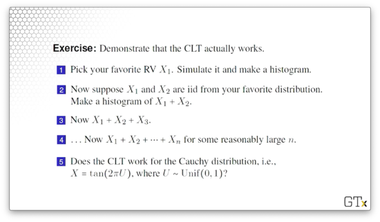
Exercises
Introduction to Estimation (OPTIONAL)
In this lesson, we are going to start our review of basic statistics. In particular, we are going to talk about unbiased estimation and mean squared error.
Statistic Definition
A statistic is a function of the observations X1,...,Xn that is not explicitly dependent on any unknown parameters. For example, the sample mean, Xˉ, and the sample variance, S2, are two statistics:
Xˉ=S2=n1i=1∑nXin−11i=1∑x(Xi−Xˉ)2
Statistics are random variables. In other words, if we take two different samples, we should expect to see two different values for a given statistic.
We usually use statistics to estimate some unknown parameter from the underlying probability distribution of the Xi's. For instance, we use the sample mean, Xˉ, to estimate the true mean, μ, of the underlying distribution, which we won't normally know. If μ is the true mean, then we can take a bunch of samples and use Xˉ to estimate μ. We know, via the law of large numbers that, as n→∞, Xˉ→μ.
Point Estimator
Let's suppose that we have a collection of iid random variables, X1,...,Xn. Let T(X)≡T(X1,...,Xn) be a function that we can compute based only on the observations. Therefore, T(X) is a statistic. If we use T(X) to estimate some unknown parameter θ, then T(X) is known as a point estimator for θ.
For example, Xˉ is usually a point estimator for the true mean, μ=E[Xi], and S2 is often a point estimator for the true variance, σ2=Var(X).
T(X) should have specific properties:
Its expected value should equal the parameter it's trying to estimate. This property is known as unbiasedness.
It should have a low variance. It doesn't do us any good if T(X) is bouncing around depending on the sample we take.
Unbiasedness
We say that T(X) is unbiased for θ if E[T(X)]=θ. For example, suppose that random variables, X1,...,Xn are iid anything with mean μ. Then:
Since E[Xˉ]=μ, Xˉ is always unbiased for μ. That's why we call it the sample mean.
Similarly, suppose we have random variables, X1,...,Xn which are iid Exp(λ). Then, Xˉ is unbiased for μ=E[Xi]=1/λ. Even though λ is unknown, we know that Xˉ is a good estimator for 1/λ.
Be careful, though. Just because Xˉ is unbiased for 1/λ does not mean that 1/Xˉ is unbiased for λ: E[1/Xˉ]=1/E[Xˉ]=λ. In fact, 1/Xˉ is biased for λ in this exponential case.
Here's another example. Suppose that random variables, X1,...,Xn are iid anything with mean μ and variance σ2. Then:
E[S2]=E[n−1∑i=1n(Xi−Xˉ)2]=Var(Xi)=σ2
Since E[S2]=σ2, S2 is always unbiased for σ2. That's why we called it the sample variance.
For example, suppose random variables X1,...,Xn are iid Exp(λ). Then S2 is unbiased for Var(Xi)=1/λ2.
Let's give a proof for the unbiasedness of S2 as an estimate for σ2. First, let's convert S2 into a better form:
Remember that Xˉ represents the average of all the Xi's: ∑Xi/n. Thus, if we just sum the Xi's and don't divide by n, we have a quantity equal to nXˉ:
Unfortunately, while S2 is unbiased for the variance σ2, S is biased for the standard deviation σ.
Example
Suppose that we have n random variables, X1,...,Xn∼iidUnif(0,θ). We know that our observations have a lower bound of 0, but we don't know the value of the upper bound, θ. As is often the case, we sample many observations from the distribution and use that sample to estimate the unknown parameter.
Consider two estimators for θ:
Y1Y2≡2Xˉ≡nn+11≤i≤XimaxXi
Let's look at the first estimator. We know that E[Y1]=2E[Xˉ], by definition. Similarly, we know that 2E[Xˉ]=2E[Xi], since Xˉ is always unbiased for the mean. Recall how we compute the expected value for a uniform random variable:
E[A]=(b−a)/2,A∼Unif(a,b)
Therefore:
2E[Xi]=2(2θ−0)=θ=E[Y1]
As we can see, Y1 is unbiased for θ.
It's also the case that Y2 is unbiased, but it takes more work to demonstrate. As a first step, take the cdf of the maximum of the Xi's, M≡maxiXi. Here's what P(M≤y) looks like:
P(M≤y)=P(X1≤y and X2≤y and … and Xn≤y)
If M≤y, and M is the maximum, then P(M≤y) is the probability that all the Xi's are less than y. Since the Xi's are independent, we can take the product of the individual probabilities:
P(M≤y)=i=i∏nP(Xi≤y)=[P(X1≤y)]n
Now, we know, by definition, that the cdf is the integral of the pdf. Remember that the pdf for a uniform distribution, Unif(a,b), is:
f(x)=b−a1,a<x<b
Let's rewrite P(M≤y):
P(M≤y)=[∫0yfX1(x)dx]n=[∫0yθ1dx]n=(θy)n
Again, we know that the pdf is the derivative of the cdf, so:
fM(y)=FM(y)dy=dydθnyn=θnnyn−1
With the pdf in hand, we can get the expected value of M:
Note that E[M]=θ, so M is not an unbiased estimator for θ. However, remember how we defined Y2:
Y2≡nn+11≤i≤XimaxXi
Thus:
E[Y2]=nn+1E[M]=nn+1(n+1nθ)=θ
Therefore, Y2 is unbiased for θ.
Both indicators are unbiased, so which is better? Let's compare variances now. After similar algebra, we see:
Var(Y1)=3nθ2,Var(Y2)=n(n+2)θ2
Since the variance of Y2 involves dividing by n2, while the variance of Y1 only divides by n, Y2 has a much lower variance than Y1 and is, therefore, the better indicator.
Bias and Mean Squared Error
The bias of an estimator, T[X], is the difference between the estimator's expected value and the value of the parameter its trying to estimate: Bias(T)≡E[T]−θ. When E[T]=θ, then the bias is 0 and the estimator is unbiased.
The mean squared error of an estimator, T[X], the expected value of the squared deviation of the estimator from the parameter: MSE(T)≡E[(T−θ)2].
Remember the equation for variance:
Var(X)=E[X2]−(E[X])2
Using this equation, we can rewrite MSE(T):
MSE(T)=E[(T−θ)2]=Var(T)+(E[T]−θ)2=Var(T)+Bias2
Usually, we use mean squared error to evaluate estimators. As a result, when selecting between multiple estimators, we might not choose the unbiased estimator, so long as that estimator's MSE is the lowest among the options.
Relative Efficiency
The relative efficiency of one estimator, T1, to another, T2, is the ratio of the mean squared errors: MSE(T1)/MSE(T2). If the relative efficiency is less than one, we want T1; otherwise, we want T2.
Let's compute the relative efficiency of the two estimators we used in the previous example:
Y1Y2≡2Xˉ≡nn+11≤i≤XimaxXi
Remember that both estimators are unbiased, so the bias is zero by definition. As a result, the mean squared errors of the two estimators is determined solely by the variance:
The relative efficiency is greater than one for all n>1, so Y2 is the better estimator just about all the time.
Maximum Likelihood Estimation (OPTIONAL)
In this lesson, we are going to talk about maximum likelihood estimation, which is perhaps the most important point estimation method. It's a very flexible technique that many software packages use to help estimate parameters from various distributions.
Likelihood Function and Maximum Likelihood Estimator
Consider an iid random sample, X1,...,Xn, where each Xi has pdf/pmf f(x). Additionally, suppose that θ is some unknown parameter from Xi that we would like to estimate. We can define a likelihood function, L(θ) as:
L(θ)≡i=1∏nf(xi)
The maximum likelihood estimator (MLE) of θ is the value of θ that maximizes L(θ). The MLE is a function of the Xi's and is itself a random variable.
Example
Consider a random sample, X1,...,Xn∼iidExp(λ). Find the MLE for λ. Note that, in this case, λ, is taking the place of the abstract parameter, θ. Now:
L(λ)≡i=1∏nf(xi)
We know that exponential random variables have the following pdf:
f(x,λ)=λe−λx
Therefore:
L(λ)≡i=1∏nλe−λxi
Let's expand the product:
L(λ)=(λe−λx1)∗(λe−λx2)∗⋯∗(λe−λxn)
We can pull out a λn term:
L(λ)=λn∗(e−λx1)∗(e−λx2)∗⋯∗(e−λxn)
Remember what happens to exponents when we multiply bases:
ax∗ay=ax+y
Let's apply this to our product (and we can swap in exp notation to make things easier to read):
L(λ)=λnexp[−λi=1∑nxi]
Now, we need to maximize L(λ) with respect to λ. We could take the derivative of L(λ), but we can use a trick! Since the natural log function is one-to-one, the λ that maximizes L(λ) also maximizes ln(L(λ)). Let's take the natural log of L(λ):
Finally, we set the derivative equal to 0 and solve for λ:
0≡λnλnλλ−i=1∑nxi=i=1∑nxi=∑i=1nxin=Xˉ1
Thus, the maximum likelihood estimator for λ is 1/Xˉ, which makes a lot of sense. The mean of the exponential distribution is 1/λ, and we usually estimate that mean by Xˉ. Since Xˉ is a good estimator for λ, it stands to reason that a good estimator for λ is 1/Xˉ.
Conventionally, we put a "hat" over the λ that maximizes the likelihood function to indicate that it is the MLE. Such notation looks like this: λ^.
Note that we went from "little x's", xi, to "big x", Xˉ, in the equation. We do this to indicate that λ^ is a random variable.
Just to be careful, we probably should have performed a second-derivative test on the function, ln(L(λ)), to ensure that we found a maximum likelihood estimator and not a minimum likelihood estimator.
Invariance Property of MLE's
If θ^ is the MLE of some parameter, θ, and h(⋅) is a 1:1 function, then h(θ^) is the MLE of h(θ).
For example, suppose we have a random sample, X1,...,Xn∼iidExp(λ). The survival function, Fˉ(x), is:
Fˉ(x)=P(X>x)=1−F(x)=1−(1−e−λx)=e−λx
In addition, we saw that the MLE for λ is λ^=1/Xˉ. Therefore, using the invariance property, we can see that the MLE for Fˉ(x) is Fˉ(λ^):
Fˉ^(x)=e−λ^x=e−x/Xˉ
Confidence Intervals (OPTIONAL)
In this lesson, we are going to expand on the idea of point estimators for parameters and look at confidence intervals. We will use confidence intervals through this course, especially when we look at output analysis.
Important Distributions
Suppose we have a random sample, Z1,Z2,...,Zk, that is iid Nor(0,1). Then, Y=∑i=1kZi2 has the χ2 distribution with kdegrees of freedom. We can express Y as Y∼χ2(k), and Y has an expected value of k and a variance of 2k.
If Z∼Nor(0,1),Y∼χ2k, and Z and Y are independent, then T=Z/Y/k has the Student's t distribution with k degrees of freedom. We can express T as T∼t(k). Note that t(1) is the Cauchy distribution.
If Y1∼χ2(m),Y2∼χ2(n), and Y1 and Y2 are independent, then F=(Y1/m)/(Y2/n) has the F distribution with m and n degrees of freedom. Notation: F∼F(m,n).
We can use these distributions to construct confidence intervals for μ and σ2 under a variety of assumptions.
Confidence Interval
A 100(1−α)% two-sided confidence interval for an unknown parameter, θ, is a random interval, [L,U], such that P(L≤θ≤U)=1−α.
Here is an example of a confidence interval. We might say that we believe that the proportion of people voting for some candidate is between 47% and 51%, and we believe that statement to be true with probability 0.95.
Common Confidence Intervals
Suppose that we know the variance of a distribution, σ2. Then a 100(1−α)% confidence interval for μ is:
Xˉn−zα/2nσ2≤μ≤Xˉn+zα/2nσ2
Notice the structure of the inequality here: Xˉn−H≤μ≤Xˉn+H. The expression H, known as the half-length, is almost always a product of a constant and the square root of S2/n. In this rare case, since we know σ2, we can use it directly.
What is z? zγ is the 1−γ quantile of the standard normal distribution, which we can look up:
zγ≡Φ−1(1−γ)
Let's look at another example. If σ2 is unknown, then a 100(1−α)% confidence interval for μ is:
Xˉn−tα/2,n−1nS2≤μ≤Xˉn+tα/2,n−1nS2
This example looks very similar to the previous example except that we are using S2 (because we don't know σ2), and we are using a t quantile instead of a normal quantile. Note that tγ,ν is the 1−γ quantile of the t(ν) distribution.
Finally, let's look at the 100(1−α)% confidence interval for σ2:
χ2α,n−12(n−1)S2≤σ2≤χ1−2α,n−12(n−1)S2
Note that χγ,ν2 is the 1−γ quantile of the χ2(ν) distribution.
Example
We are going to look at a sample of 20 residual flame times, in seconds, of treated specimens of children's nightwear, where a residual flame time measures how long it takes for something to burst into flames. Don't worry; there were no children in the nightwear during this experiment.
Let's compute a 95% confidence interval for the mean residual flame time. After performing the necessary algebra, we can calculate the following statistics:
Xˉ=9.8475,S=0.0954
Remember the equation for computing confidence intervals for μ when σ2 is unknown:
Xˉn−tα/2,n−1nS2≤μ≤Xˉn+tα/2,n−1nS2
Since we are constructing a 95% confidence interval, α=0.05 Additionally, since we have 20 samples, n=20. Let's plug in:
After the final arithmetic, we see that the confidence interval is:
9.8029≤μ≤9.8921
We would say that we are 95% confident that the true mean, μ, (of the underlying distribution from which our 20 observations were sampled) is between 9.8029 and 9.8921.
OMSCS Notes is made with
in NYC by Matt Schlenker.