Simulation
Output Data Analysis
56 minute read
Notice a tyop typo? Please submit an issue or open a PR.
Output Data Analysis
Introduction
Let's recall the steps that we take when performing a simulation study. First, we conduct a preliminary analysis of the system. Then, we build models. Third, we verify and validate our models and their implementations, potentially returning to previous steps depending on the outcome. Next, we design experiments, conduct simulation runs, and perform statistical analysis of the output. Finally, we implement our solutions.
Don't forget to analyze simulation output!
Why Worry about Output?
Since the input processes driving a simulation - interarrival times, service times, breakdown times, etc. - are random variables, we must regard the simulation's output as random.
As a result, simulation runs only yield estimates of measures of system performance. For example, we might run our simulation many times and arrive at an estimate for the mean customer waiting time. We derive these estimates from observations output by the simulation.
Since the output is random, the estimators are also random variables. Therefore, they are subject to sampling error, which we must consider to make valid inferences about system performance.
For example, we wouldn't want to run a simulation several times and then report just the average value for a particular metric. Ideally, we'd like to present a confidence interval that presents a range of likely values.
Measures of Interest
We might be interested in means. For example, if we are simulating a waiting room, we might be very curious about the mean waiting time.
We also have to look at variances. Again, if we are simulating a waiting room, we should look at how much waiting time is liable to vary from customer to customer.
Quantiles can also be very important, especially in the domain of risk analysis. For example, we might want to know the 99% quantile for waiting time in a particular queue.
We could be interested in success probabilities. We might want to know the probability that a particular job finishes before a certain time.
Additionally, we want to have point estimators and confidence intervals for the various statistics above.
The Problem
The problem is that simulations rarely produce raw input that is independent and identically distributed. We have to be careful about how we analyze data since we cannot make this iid assumption.
For example, let's consider customer waiting times from a queueing system. These observations are not independent - typically, they are serially correlated. If one customer has to wait a long time, we expect the person next to them to have to wait a long time as well.
Additionally, these observations are not identically distributed. Customers showing up early in the morning are likely to have much shorter waiting times than those who arrive during peak hours.
Furthermore, these observations are not even normally distributed. Waiting times skew right - occasionally, we have to wait a very long time - and they certainly cannot be negative.
As a result, we can't apply the classical statistical techniques to the analysis of simulation output. We will focus on other methods to perform statistical analysis of output from discrete-event computer simulations.
If we conduct improper statistical analysis of our output, we can invalidate any results we may wish to present. Conversely, if we give the output the proper treatment, we may uncover something important. Finally, if we want to study further, there are many exciting research problems to explore.
Types of Simulation
There are two types of simulations we will discuss with respect to output analysis.
When we look at finite-horizon or terminating simulations, we look at the short-term performance of systems with a defined beginning and end. In steady-state simulations, we are interested in the performance of a long-running system.
Finite-Horizon Simulations
A finite-horizon simulation ends at a specific time or because of a specific event. For instance, if we are simulating a mass-transit system during rush hour, the simulation ends when rush hour ends. If we are simulating a distribution system for one month, the simulation ends when the month ends. Other examples of finite-horizon simulations include simulating a production system until a set of machines breaks down or simulating the start-up phase of a system.
Steady-State Simulations
The purpose of a steady-state simulation is to study the long-run behavior of a system. A performance measure in such a system might be a parameter characteristic of the process's long-term equilibrium. For instance, we might be interested in a continuously operating communication system where the objective is the computation of the mean delay of a packet in the long run.
A Mathematical Interlude (OPTIONAL)
In this lesson, we will look at some math that informs why we cannot give simulation output the classical statistical treatment.
A Mathematical Interlude
We'll look at a few examples illustrating the fact that results look a little different when we don't have iid observations. Like we've said, we have to be careful.
Let's talk about our working assumptions. For the remainder of this lesson, let's assume that our observations, , are identically distributed with mean , but are not independent. Such an assumption often applies in the context of steady-state simulation.
We'll compute the sample mean and sample variance, which we know are very effective estimators when the observations are iid. As we will see, the sample mean still works well, but we'll have to be careful regarding the sample variance.
Properties of the Sample Mean
Let's look at the expected value of the sample mean, :
Since , . Therefore, the sample mean is still unbiased for . We already knew this: the sample mean is always unbiased for so long as all of the observations come from a distribution with mean , regardless of whether they are correlated with one another.
Now let's consider the covariance function, which we define as :
We also know that, by definition, the variance of a random variable is equal to the covariance of that random variable with itself:
Thus, we can create an expression for the variance of the sample mean:
We can re-express the covariance of the sample mean using the definition of the sample mean. Notice that we have two summation expressions, and we divide by twice:
By definition of , we can replace with :
Notice that we take the absolute value of to prevent a negative value for . After a bunch of algebra, equation simplifies to a single summation expression:
How did we get from to ? Let's take all of the pairs and build an covariance matrix.
Let's look at the first row. These values correspond to pairs. For instance, the first cell in the row is the pair, which, using the notation, is . We continue to increment the 's until we reach , which has a corresponding value of .
Similarly, we can see that the second row corresponds to pairs, the th row corresponds to pairs, the first column corresponds to pairs, and the last column corresponds to pairs.
We can see that there are terms, since we have an matrix. How many terms do we have? If we shift the diagonal above the diagonal down by one row, we see that we have terms. If we shift the diagonal below the diagonal up by one row, we see that we have another terms. In total, we have terms.
If we continue this process, we will see that we have terms, and, generally terms.
Equation above is very important because it relates the variance of the sample mean to the covariances of the process. With this in mind, let's define a new quantity, , which is times the variance of the sample mean:
We can also define the related variance parameter, , which is the limit of as goes to infinity:
Note that, as goes to infinity, the term goes to zero so:
The weird notation means that the equality holds only if the terms decrease to 0 quickly as .
If the 's are iid, then for all , we have . In that case, .
However, in the dependent case, adds in the effects of all of the pairwise, nonzero covariances. In queueing applications, these covariances are always positive, which makes sense: if we wait a long time, the person next to us probably waits a long time. As a result, , which may be much bigger than we expect.
We can think of the ratio as sort of the number of observations needed to obtain the information that is equivalent to one "independent" observation.
If , then the classical confidence interval (CI) for the mean will not be accurate, and we'll discuss this phenomenon more shortly.
Example
The first-order autoregressive process is defined by:
Note that , , and the 's are iid random variables that are independent of . The 's are all Nor(0,1) and the covariance function is defined as:
Let's apply the definition of :
After some algebra, we get the following result:
Note that . As an example, if , then . We need to collect nineteen correlated observations to have the information that we would get from just one iid observation.
Properties of the Sample Variance
Let's remember the formula for the sample variance:
If are iid, then is unbiased for . Moreover, is also unbiased for and .
If the 's are dependent, then may not be such a great estimator for , , or .
Let's again suppose that are identically distributed with mean , and correlated with covariance function .
Let's get the expected value of :
Note that, since the 's are identically distributed, :
Now, let's remember that . Therefore:
Since , then:
Let's assume that the 's are greater than zero. Remember equation from above:
Given that , we can rewrite the expected value of the sample variance as:
Let's simplify:
If the 's are positive, which we expect them to be since the 's are correlated, then:
Therefore:
In turn:
Collecting these results shows that:
As a result, we should not use to estimate . What happens if we do use it?
Let's look at the classical CI for the mean of iid normal observations with unknown variance:
Since we just showed that , the CI will have true coverage . Our confidence interval will have much less coverage than we claim that it has. This result demonstrates why we have to be very careful with correlated data.
Finite-Horizon Analysis
In this lesson, we will talk about how to deal with correlated data in the context of finite-horizon simulations using a technique called the method of independent replications.
Finite-Horizon Analysis
Our goal is to simulate some system of interest over a finite time horizon and analyze the output. For now, we will look at discrete simulation output, , where the number of observations, , can be a constant or random.
For example, we can obtain the waiting times, , of the first one hundred customers to show up at a store. In this case, is a specified constant: 100. Alternatively, could denote the random number of customers observed during a time interval, , where itself is known or random. For instance, we might consider all the customers that show up between 10 a.m. and 2 p.m. In this case, is specified, but is random. We could also consider all customers from 10 a.m. until the store owner has to leave to pick up his kid from school. In this case, is random.
We don't have to focus on only discrete output. We might observe continuous simulation output, , over an interval , where again can be known or random. For example, might denote the number of customers in the queue between 8 a.m. and 5 p.m, or it might denote the number of customers between 8 a.m. and whenever the store owner has to leave to pick his kid up. In the first case, is known; in the second, is random.
Estimating Sample Mean
We want to estimate the expected value of the sample mean of a collection of discrete observations. For example, we might be taking observations at the bank, and we might want to estimate the average waiting time for a customer. Let's call the expected value of the sample mean . Therefore:
By definition, is an unbiased estimator for because . Now, we also need to provide an estimate for the variance of . With these two estimates, we can provide a confidence interval for the true value of .
Since the 's are not necessarily iid, the variance of is not equal to . As a result, we cannot use the sample variance, , divided by to estimate . What should we do?
Method of Independent Replications
We can use the method of independent replications to estimate . This method involves conducting independent simulation runs, or replications, of the system under study, where each replication consists of observations. We can easily make the replications independent by re-initializing each replication with a different pseudo-random number seed.
We denote the sample mean from replication by:
Note that is observation from replication . Put another way, is customer 's waiting time in replication . For example, if we have five replications, each with one hundred observations, then is the twentieth observation from the third replication.
If we start each replication under the same operating conditions - all of the queues are empty and idle, for example - then the replication sample means, are iid random variables.
We can define the grand sample mean, , as the mean of the replication means:
The obvious point estimator for is the sample variance of the 's, because those observations are iid. Let's remember the definition of the sample variance:
Note that the forms of and , which we shouldn't use, resemble each other. But, since the replication sample means are iid, is usually much less biased for than is . Since the 's are iid, we can use as a reasonable estimator for the variance of .
If the number of observations per replication, , is large enough, the central limit theorem tells us that the replicate sample means, , are approximately iid Nor(. From that result, we can see that the is approximately distributed as a random variable:
From there, we have the approximate independent replications two-sided confidence interval for :
Let's recap what we did. We took replications of correlated observations, which we then transformed into iid 's. From there, we took the sample mean and the sample variance, and we were able to construct a confidence interval for .
Example
Suppose we want to estimate the expected average waiting time for the first customers at the bank on a given day. We will make independent replications, each initialized empty and idle and consisting of waiting times. Consider the following replicate means:
If we plug and chug, we can see that and . If , the corresponding t-quantile is , which gives us the following 95% confidence interval for the expected average waiting time for the first 5000 customers:
Finite-Horizon Extensions
In this lesson, we will expand the range of benefits that the method of independent replications (IR) can provide. For example, we can use IR to get smaller confidence intervals for the mean or to produce confidence intervals for things other than the mean, like quantiles.
Smaller Confidence Intervals
If we want a smaller confidence interval, we need to run more replications. Let's recall the approximate independent replications two-sided confidence interval for :
We can define the half-length of the current confidence interval as the term to the right of the plus-minus sign. We'll call that :
Suppose we would like our confidence interval to have half-length :
Note here that we are holding the variance estimator fixed based on the current number of replications - we can't look into the future. We need to find some such that our confidence interval is sufficiently narrow.
Let's solve the equation for the desired half-length for :
As we increase the degrees of freedom, the corresponding value of the -quantile decreases. Therefore, since :
So:
With a little algebra, we can see that:
So:
Using this expression, we can set , run more replications, and re-calculate the confidence interval using all reps. Our new confidence interval will have a half-length that is probably close to .
Notice the squared term in this expression: if we want to reduce the length of the confidence interval by a factor of , we will need to increase our replications by a factor of .
Quantiles
The p-quantile of a random variable, , having cdf is defined as:
If is continuous, then is the unique value such that and .
For example, let's suppose that we have a random variable . We know that has the cdf . Therefore:
We can use the method of independent replications to obtain confidence intervals for quantiles. For example, let denote the maximum waiting time that some customer experiences at the airport ticket counter between 8 a.m. and 5 p.m. during replication of a simulation, .
Let's order the iid 's: . Then, the typical point estimator for the quantile is:
In layman's terms, we retrieve the that is larger than other 's. Since we are using order statistics, we can just retrieve, essentially, the order statistic. As we have seen before, the addition is a continuity correction, and is the "round-down" function. For example, if and , we would look at the order statistic.
Now that we have a point estimator for , we can get a confidence interval for . A slightly conservative, approximate, nonparametric confidence interval will turn out to be of the form .
Let's remember that, by definition:
As a result, we can think about a single event as a Bern() trial. If we define a random variable, , as the number of 's that are less than or equal to , then:
The event means that between and of the 's are . This event is equivalent to the following expression involving the order statistics and :
Therefore:
We have a binomial expression that is equivalent to the expression on the right above:
This binomial expression is approximately equal to:
Note that is the Nor(0,1) cdf, the 0.5 terms are continuity corrections, and the approximation requires that .
To get the approximate confidence interval of the form , we need to find and such that:
How do we choose and ? We can set:
After some algebra:
Remember that we need the floor and ceiling function here because and must be integers.
Note that if we want to get reasonably small half-lengths for "extreme" () quantiles, we will likely need to run a huge number of replications.
Example
Let's suppose that we want a confidence interval for and we've made replications. The point estimator for is:
With the confidence interval in mind, let's compute and :
As a result, the confidence interval for the quantile is , and the point estimator is .
Simulation Initialization Issues
In this lesson, we will look at how to start a simulation and when to start keeping data for steady-state analysis.
Introduction
Before running a simulation, we must provide initial values for all of the simulation's state variables. We might not know appropriate initial values for these variables, so we might choose them arbitrarily. As always, we have to be careful. Such a choice can have a significant but unrecognized impact on the simulation run's outcome.
For example, it might be convenient to initialize a queue as empty and idle, but that might not be the best choice. What if the store that we are modeling is having a sale, and there is a long line already formed by the time the store opens?
This problem of initialization bias can lead to errors, particularly in steady-state output analysis.
Some Initialization Issues
Visual detection of initialization effects is sometimes very difficult. For example, queuing systems have high intrinsic variance, and it can be hard to see the initialization effects through the noise of the variance.
We have to think about how we should initialize a simulation. For example, suppose a machine shop closes at a certain time each day. There might be customers remaining at the end of the day, and we have to make sure that the next day starts with those customers in mind.
Initialization bias can lead to point estimators for steady-state parameters that have a high mean-squared error and confidence intervals that have poor coverage, all because the initialization is not representative of the steady-state.
Detecting Initialization Bias
We can try to detect initialization bias visually by scanning the simulation output. However, this approach is not simple: the analysis is tedious, and it's easy to miss bias amidst general random noise.
To make the analysis more efficient, we can first transform the data - for instance, take logarithms or square roots - we can smooth it, average it across several replications, or apply other strategies to illuminate bias.
We can also conduct formal statistical tests for initialization bias. For example, we might conduct a test to see if the mean or variance of a process changes over time. If it does, then the process was not completely in steady-state when we began to collect observations.
Dealing with Bias
We can truncate the output by allowing the simulation to "warm up" before retaining data. Ideally, we want the remaining data to be representative of the steady-state system. Output truncation is the most popular method for dealing with bias, and most simulation languages have built-in truncation functions.
We have to be careful when selecting a truncation point. If we truncate the output too early, then significant bias might still exist in our retained data. If we truncate the output too late, we end up wasting good steady-state observations.
To make matters worse, all simple rules to give truncation points do not perform well in general. However, a reasonable practice is to average the observations across several replications and then visually choose a truncation point. There are also newer, sophisticated, sequential change-point detection algorithms that are proving to be useful.
Example
We want to select a truncation point somewhere in the following series of observations.
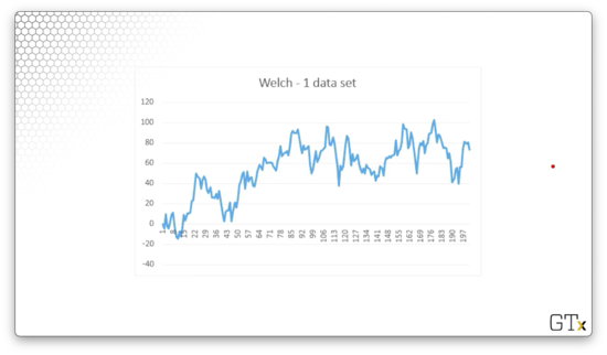
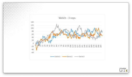
Let's run three replications and look at the resulting data.
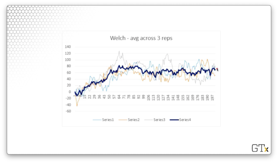
Let's average the observations across the three replications.
We can even smooth out the average using moving averages.
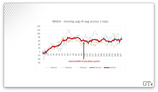
Here we can identify what looks like a reasonable truncation point. We'd start retaining observations from this point forward.
Dealing with Bias, Again
As an alternative, we could take an extremely long simulation run to overwhelm the initialization effects. This strategy is conceptually simple to carry out and may yield point estimators having lower mean-squared error than the truncation method. However, this approach can be wasteful with observations. In other words, we might need an excessively long run before the initialization effects become negligible.
Steady-State Analysis
In this lesson, we will introduce steady-state simulation analysis and the method of batch means.
Steady-State Analysis
Let's assume that we have removed our initialization bias, and we have steady-state, or stationary, simulation output . Our goal is to use this output to estimate some parameter of interest, such as the mean customer waiting time or the expected profit produced by a certain factory configuration.
In particular, suppose the mean of this output is the unknown quantity . Like we've seen in the past, we can use the sample mean, , to estimate . As in the case of terminating / finite-horizon simulations, we must accompany the value of any point estimator with a measure of its variance. In other words, we need to provide an estimate for .
Instead of estimating directly, we can estimate the variance parameter, which is basically equivalent:
Remember that, if the observations are correlated, then is equal to the following:
If the 's decrease quickly as , then is just the sum of the covariances:
The quantity shows up all over the place, from simulation output analysis to Brownian motions to financial engineering applications, and more.
For example, consider a MA(1) process, , where the 's are iid Nor(0,1). We determined that , , and . Therefore:
As another example, consider an AR(1) process, , where the 's are iid , , and . For this process, . We determined that , so as .
Many methods exist for estimating and conducting steady-state output analysis in general, such as:
- batch means
- independent replications
- standardized time series
- spectral analysis
- regeneration
- ARMA time series modeling
Method of Batch Means
We can use the method of batch means (BM) to estimate and calculate confidence intervals for . We divide one long simulation run into several contiguous batches and then appeal to a central limit theorem to assume that the resulting batch sample means are approximately iid normal.
In particular, suppose we partition our observations, , into nonoverlapping, contiguous batches, each consisting of observations. Therefore, . For example, the first batch contains the observations , the second batch contains the observations , and the th batch contains the observations .
We can admit that the observations at the end of batch and the beginning of batch are slightly correlated. Still, we can treat just about all of the observations across batches as being independent.
The th batch mean is the sample mean of the observations from batch :
Batch begins at observation and ends at . If we divide the observations by , we have computed the sample mean.
The batch means are correlated for small , but, for large :
Similar to the method of independent replications, we can define the batch means estimator for as:
We can see that looks a lot like the sample variance of the batch means. Notice the in the numerator. Since we defined as the limit of , we need to include the in the estimator. We can also see that is also approximately distributed as a random variable:
How good is as an estimator for ? Let's look at the expected value:
Since , then , so is asymptotically unbiased for as the batch size .
Properties of Batch Means (OPTIONAL)
In this lesson, we will look at some properties of the batch means estimator for as well as the batch means confidence interval for the steady-state mean. This confidence interval is the key result in steady-state analysis, if not output analysis as a whole.
Estimator
Let's recall the batch means estimator for :
Here, is the batch size, and is the number of batches, is the sample size, is the th batch mean, and is the sample mean. As we saw last time, is approximately distributed as a random variable:
How good is as an estimator of ? Let's look at its mean and variance. As we saw last time:
Since the estimator's expected value equals the value it estimates, is asymptotically unbiased for as .
More-Precise Result
It turns out that we can come up with a more precise definition for the expected value of :
We don't particularly care about the function, as it goes to zero faster than as gets big.
However, the middle term doesn't go away as quickly, and it's a first-order bias term. The good news is that whatever the number of batches, , this term decreases as the batch size, , gets big.
Let's look at the definition of , which is a function of the covariances:
Let's look at the variance of our estimator:
Mean-Squared Error of
These facts immediately imply that, for large and :
Of course, for large , , so:
Our goal is to find the best choice of and , subject to the constraint , so as to minimize the MSE.
Let's fix for now and find the appropriate value for . To do so, lets take , where and .
We know that so:
Therefore:
If we choose any , one of the two terms will converge to zero more slowly than the other. If we choose , both terms will converge to zero by . Therefore:
If we minimize the above expression with respect to , we get the "optimal" batch size:
Furthermore, if we plug in back into the mean-squared error equation, we get the optimal mean-squared error:
Unfortunately, and are not known in practice and must be estimated somehow to produce a concrete value for and . We will save this estimation for another day. Nevertheless, we can see that we need a batch size on the order of to minimize the MSE.
Batch Means Confidence Interval
Let's turn now to the batch means confidence interval for . Since the batch means for large , we have the following approximate confidence interval for :
This result is very similar to the confidence interval we saw with the method of independent replications. The difference is that the method of batch means divides one long run into many batches, whereas the method of independent replications uses many independent shorter runs.
If we consider the old independent replications numerical example, but now pretend that the 's are batch means instead of replicate means, then the same numbers carry through the example if we note that .
Some Properties of Batch Means CI
Let's define the half-length of the confidence interval as:
As , we can show that:
Note that we are working with the distribution here, not our familiar distribution.
The expected value of decreases as a function of the number of batches, . However, the decrease smoothes out around . A common recommendation is to take and concentrate on increasing the batch size as much as possible.
The technique of batch means is intuitively appealing and easy to understand. However, problems arise when the 's are not stationary, which may arise if significant initialization bias is present, the batch means are not normal, or if the batch means are not independent.
If any of these assumption violations exist, poor confidence interval coverage may result, unbeknownst to us. To fix the initialization bias problem, we can truncate some of the data or make a longer simulation run, as discussed previously. To fix the lack of independence or normality of the batch means, we can increase the batch size, .
Other Steady-State Methods
In this lesson, we will look at a few variance estimators and confidence intervals that provide even better results than the method of batch means. One of the techniques we will discuss is the method of overlapping batch means.
Independent Replications
Of all the difficulties that we might encounter when using the method of batch means, the possibility of correlation among the batch means might be the most troublesome. Of course, we can decrease the likelihood of this correlation by increasing the batch size, , but it remains an issue.
The method of independent replications described earlier in the context of terminating simulations explicitly avoids this problem. As it turns out, we can use replicate means in steady-state analysis, too.
Unfortunately, since each of the reps has to be started properly, we have to deal with initialization bias times instead of the one time we have to deal with it if we opt for the method of batch means. Because of this compounded risk of initialization bias, the recommendation is to use batch means over independent replications for steady-state analysis.
Overlapping Batch Means
Suppose that we have the following overlapping batches:
Let's look at the formula for the overlapping batch means:
We can see, for example, that if , the corresponding batch mean averages observations . For , the batch mean averages , and so forth.
As we might expect, the overlapping batch means are highly correlated. No problem! The overlapping batch means estimator for is and the estimator for is:
As the run length, , and the batch size, , get large:
What this result tells us is that the expected value of both variance estimators approaches , but the variance of the overlapping batch means estimator is smaller than that of the batch means estimator: the former is two-thirds the size of the latter. So, overlapping batch means has the same bias but lower variance than the regular batch means. Note that we did not attempt to make the overlapping batch means independent.
This result is related to the fact that is almost identical to what is known as Bartlett's spectral estimator for .
For large and , it can be shown that:
From this result, we can see that we get more degrees of freedom than in regular batch means. We have the corresponding confidence interval:
Here's a recommendation: for large and , use overlapping batch means instead of batch means!
Spectral Estimation
Spectral estimation estimates the variance of , as well as the analogous confidence intervals for in a completely different manner than that of batch means. This approach uses the so-called frequency domain, whereas batch means uses the time domain. Spectral estimation sometimes takes a little effort, but it works well. For more information, check out this reference.
Regeneration
Many simulations can be broken into iid blocks or sets that probabilistically "start over" at certain regeneration points. It's like the simulation begins from scratch.
For instance, consider an M/M/1 queue's waiting time process. These iid blocks could be defined by groups of customers whose endpoints have zero waiting times. When we encounter a customer that doesn't have to wait, it's almost like the simulation has restarted.
Regeneration uses this iid structure and, under certain conditions, gives great estimators for the variance of along with confidence intervals for .
The method effectively eliminates any initialization problems because each block appears to be in a steady state. On the other hand, it may be difficult to define natural regeneration points, and extremely long simulation runs are often needed to obtain a reasonable number of iid blocks.
Standardized Time Series
This technique uses a very sophisticated central limit theorem to standardize an entire process into a collection of normal random variables. We can use a process central limit theorem to standardize a stationary simulation process into a Brownian bridge process.
The properties of Brownian bridges are then used to calculate several good estimators for the variance of and the confidence intervals for . This method is easy to apply and has some asymptotic advantages over batch means.
Combining various strategies to obtain even better variance estimators is a hot research topic these days.
OMSCS Notes is made with in NYC by Matt Schlenker.
Copyright © 2019-2023. All rights reserved.
privacy policy