Statistical Analysis of Time Series

Global Statistics

In this lesson, we are going to look at the various types of statistics that we can take on time series data.

Let's consider our old DataFrame df from a previous lecture.

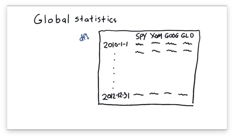
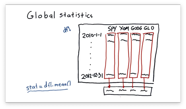
We can take the mean of each column in df like this:

df1.mean()

This statement will create a new one-dimensional ndarray whose elements are the means of the columns in df.

DataFrames contain many helpful statistical methods, and some common ones are listed below.

df.mean()
df.median()
df.mode()
df.std() # Standard Deviation
df.sum() # Column-wise sum of elements
df.prod() # Column-wise product of elements
# And many others!

Documentation

Computations / descriptive stats

Compute Global Statistics

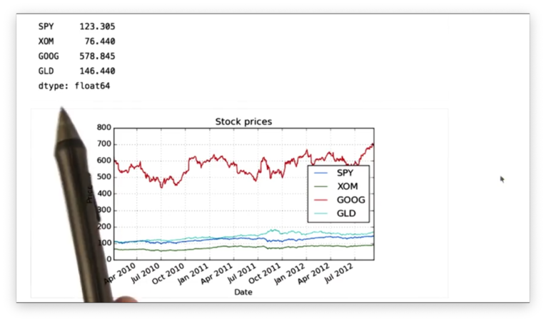
Given our DataFrame df that contains stock data for SPY, XOM, GOOG, and GLD, we can retrieve the mean price for each stock with the following code:

df.mean()

If we print the means, we see the following.

Similarly, we can compute the median price of each stock:

df.median()

Recall that while the mean is the average value - the sum of all elements divided by the number of elements - the median is the middle value. That is, given a sorted dataset, the median value is the value such that an equal number of values come before and after.

If we print out the median price for each stock, we see the following.

Additionally, we can compute the standard deviation of the prices of each stock:

df.std()

Mathematically, the standard deviation is the square root of the variance. Intuitively, the standard deviation is a measure of deviation from a central value; in this case, the central value is the mean.

If we print out the standard deviation of the prices of each stock, we see the following.

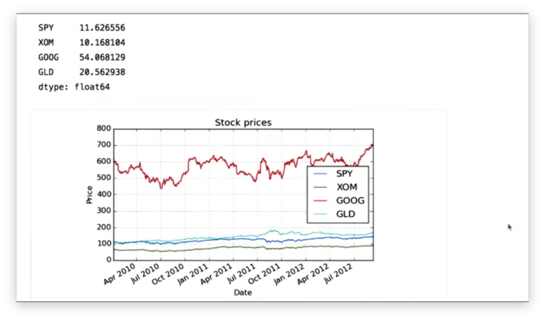
We can see that GOOG has the highest standard deviation among the stocks. This means the price of GOOG has varied more over time than the price of the other stocks.

Documentation

Rolling Statistics

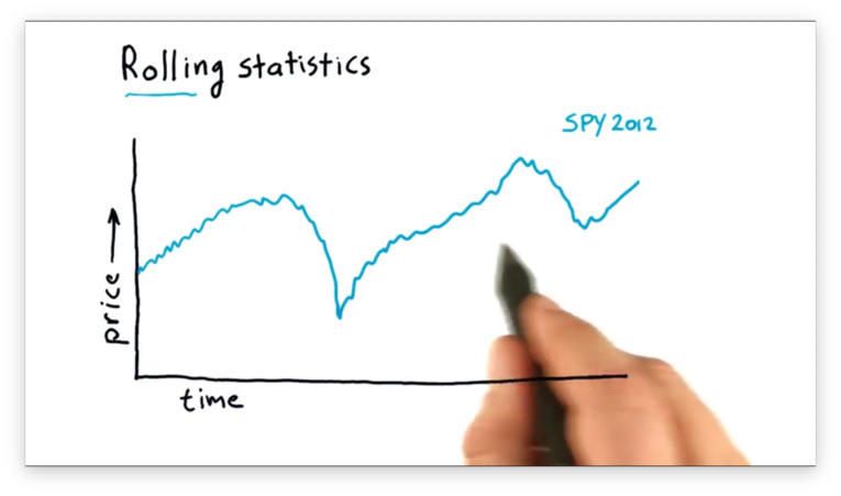
Let's talk about a new kind of statistics: rolling statistics. Instead of computing a single statistic over an entire set of data, we compute a rolling statistic against a subset, or window, of that data, and we adjust the window with each new data point we encounter.

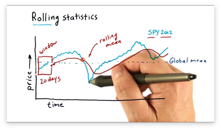
Consider the following graph of SPY price data.

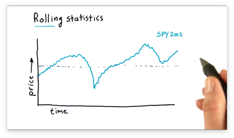
We can compute the global mean of this data set, which is a single value described by the line below.

We can also compute an n-day rolling mean. For a given day d, the n-day rolling mean is equal to the mean of the d - (n - 1) through d days. The window is the parameter n.

For example, we can compute a 20-day rolling mean as follows. For a given day d, the 20-day rolling mean is equal to the mean of the d - 19 through d days. The window here is 20.

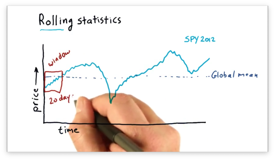
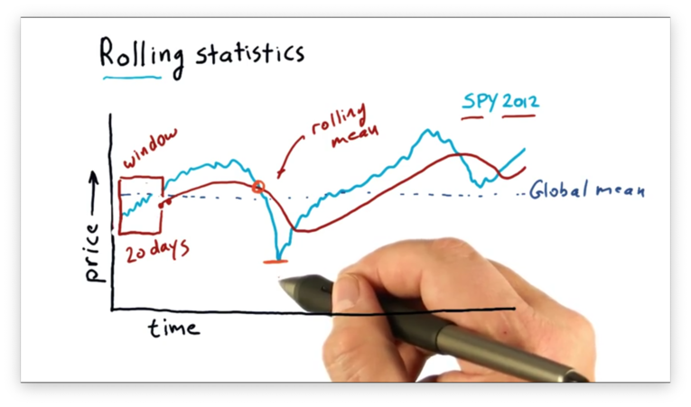
We can calculate the 20-day rolling mean for day d' = d + 1 as the mean of the d - 18 through d + 1 days. Generally, we can imagine "sliding" the window through the data set and computing the rolling mean at each data point.

Note that our sliding mean calculations form a curve that begins 20 data points after the beginning of the SPY data.

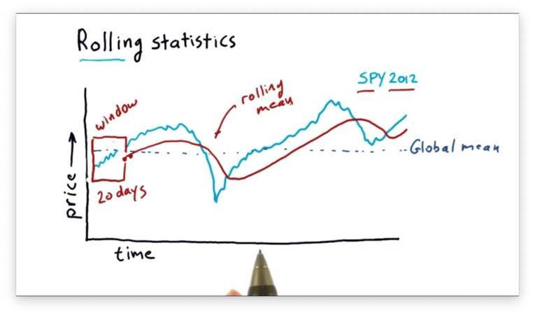
We can see that this rolling mean line follows the day-to-day values of the SPY price data, but it lags slightly as it has to incorporate the past twenty days into its calculation.

The rolling mean is referred to as a simple moving average (SMA) by technical analysts. Technical analysts utilize SMAs by looking at points where the price crosses over the SMA.

A hypothesis that many technical analysts abide by is that the rolling mean may be a good representation of the true, underlying price of the stock and that significant deviations from that mean eventually result in a return to the mean.

As a result, if you can spot significant deviations from the mean, you might be able to spot a buying opportunity.

A challenge to this strategy, though, is understanding when a deviation is significant enough to warrant attention. Small deviations may be noise more often than not.

Which Statistic to Use Quiz

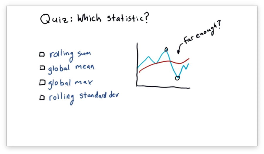
Assume we are using a rolling mean to track the movement of a stock. We are looking for an opportunity to find when the price has diverged significantly far from the rolling mean, as we can use this divergence to signal a buy or a sell.

Which statistic might we use to discover if the price has diverged significantly enough?

Which Statistic to Use Quiz Solution

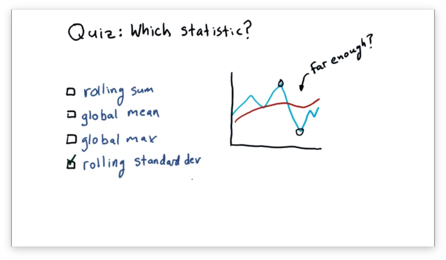
Standard deviation gives us a measure of divergence from the mean. Therefore, if the price breaches the standard deviation, we may conclude that the price has moved significantly enough for us to consider buying or selling the stock.

Bollinger Bands

How can we know if a deviation from the rolling mean is significant enough to warrant a trading signal? In the 1980s, John Bollinger created the Bollinger bands to address this question.

Bollinger reasoned that we ought to consider the recent volatility of a stock before buying or selling. If the stock is very volatile, we might discard movements above and below the rolling mean. If the stock is not very volatile, however, a similarly-sized movement might deserve our attention.

His idea was to add two bands to the graph of price movement: one that was two standard deviations above the rolling mean, and one that was two standard deviations below the rolling mean.

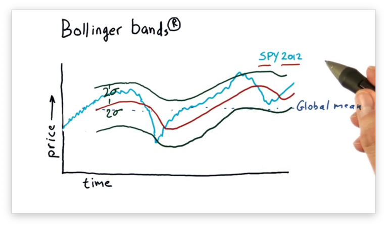
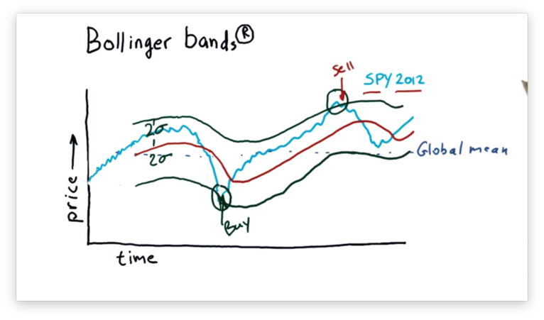
With lower band L and upper band H in place, we can devise a simple trading strategy as follows. Price movement below L followed by price movement above L signals a buy. Conversely, price movement above H followed by price movement below H signals a sell.

Computing Rolling Statistics

Pandas provides a number of functions to compute moving statistics. Given a DataFrame df and a window window, we can compute the rolling mean of the columns in a DataFrame like this:

# NOTE: this is super old syntax.
pd.rolling_mean(df, window=window)

# NOTE: this is the new syntax.
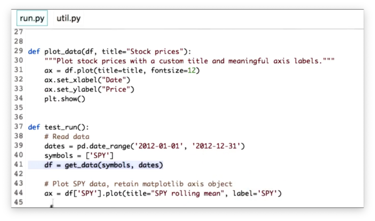
df.rolling(window).mean()

Let's look at some starter code for reading SPY data into a DataFrame df and plotting it.

We can generate an ndarray rm_SPY containing the values of a 20-day rolling mean over the SPY data:

# NOTE: this is super old syntax.
pd.rolling_mean(df['SPY'], window=20)

# NOTE: this is the new syntax.
df['SPY'].rolling(20).mean()

We can plot rm_SPY on the same plot we used for the raw price data by passing in the matplotlib axis object ax we assigned from the previous call to the plot method:

# ax = df['SPY'].plot(...)
# ...

rm_SPY.plot(label="Rolling mean", ax=ax)

Specifying the label as "Rolling mean" is useful when adding a plot legend. Let's do that now, along with some axis labels:

ax.set_xlabel('Date')
ax.set_ylabel('Price')
ax.legend(loc='upper left')

If we display the plot, we see the following.

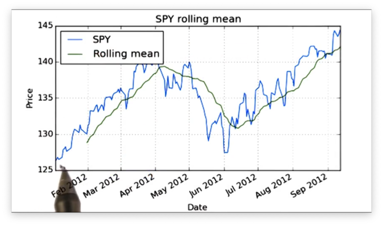
Observe that the rolling mean line has missing initial values. Since we defined a 20-day window, we can't actually compute the rolling mean until we have at least 20 days worth of pricing data.

Also observe that the rolling mean appears to track the price data, but is much smoother than the raw data.

Documentation

Calculate Bollinger Bands Quiz

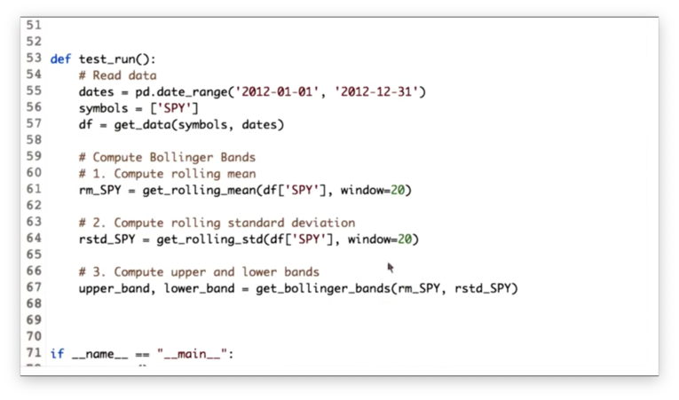
Computing Bollinger bands consists of three main steps: first, computing the rolling mean; second, computing the rolling standard deviation and; third, computing the upper and lower bands.

Our goal is to implement the three functions below to accomplish these tasks.

Calculate Bollinger Bands Quiz Solution

Given an ndarray values and a window window, we can calculate the rolling standard deviation as follows:

# OLD
pd.rolling_std(values, window=window)

# NEW
values.rolling(window).std()

Given a rolling mean rm and a rolling standard deviation rstd, we can calculate the Bollinger bands as follows:

rm + (2 * rstd), rm - (2 * rstd)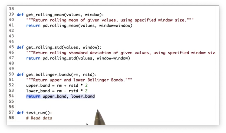

Documentation

pandas.DataFrame.rolling

Daily Returns

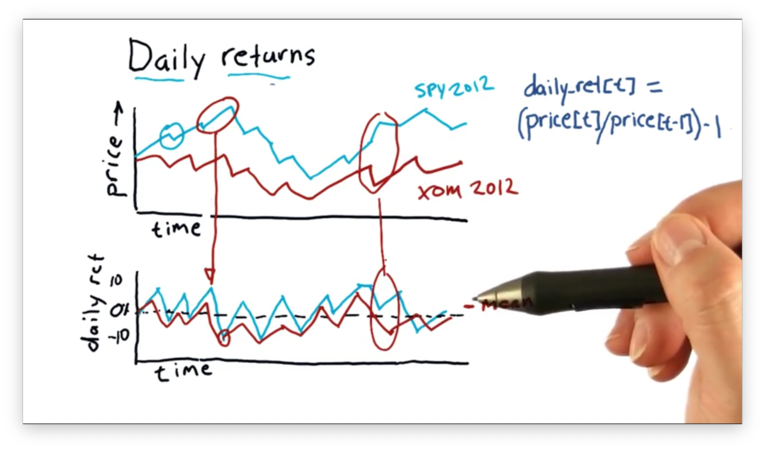
Daily returns reflect how much the price of a stock increased or decreased on a particular day. We can calculate the daily return on a given day t with a simple equation:

(price[t] / price [t - 1]) - 1

For example, let's suppose that yesterday a stock closed at $100 and today the stock closed at $110. The daily return for the stock today is:

(110 / 100) - 1 # = 1.1 - 1 = 0.1 = 10%

Here's how a chart for daily returns might look.

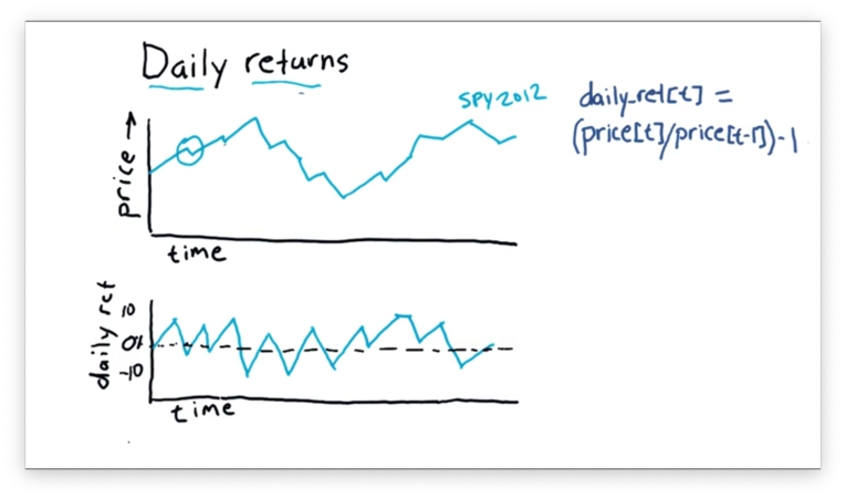
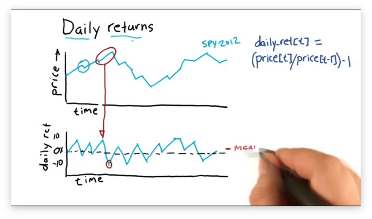
We can see the daily returns "zigzag" above and below zero, indicating that the stock finished above its previous close on some days and finished below on others.

We can also take the average over the daily return values, which, since the stock seems to have risen more days than it fell, would be slightly above zero.

Daily returns can be a helpful tool for comparing two different stocks, such as XOM (Exxon) and SPY. The following plot of daily returns reveals an unusual feature: a day where SPY had a positive daily return, and XOM had a negative daily return.

Compute Daily Returns Quiz

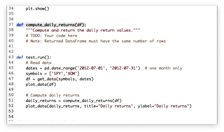
Our task is to implement a function compute_daily_returns that receives a DataFrame df and returns a DataFrame consisting of the daily return values. The returned DataFrame must have the same number of rows as df, and any rows with missing data must be filled with zeroes.

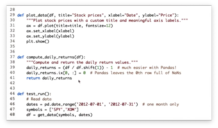
Compute Daily Returns Solution

Given a DataFrame df with n rows, we can create a new DataFrame with n + m rows where each row is shifted down m rows with the following code:

df.shift(m)

Note that the newly created m rows at the top of the DataFrame will be filled with NaN values.

Therefore, we can divide every price in our DataFrame df by the price on the previous day like this:

df / df.shift(1)

We can complete the daily return calculation, and generate a DataFrame daily_returns like so:

df / df.shift(1) - 1

The only thing we have to consider now is the first row in daily_returns. Since the first row in the shifted DataFrame is filled with NaN values, any subsequent mathematical operations on those values yield NaN.

However, our task was to fill any rows with missing data with zeroes. We can fix daily_returns like this:

# Deprecated
daily_returns.ix[0, :] = 0

# Use this
daily_returns.iloc[0] = 0

Documentation

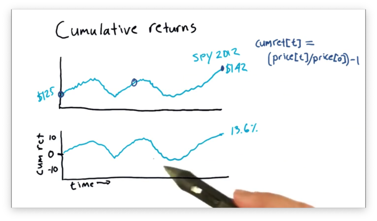
Cumulative Returns

Let's look at a chart of SPY prices for the year 2012.

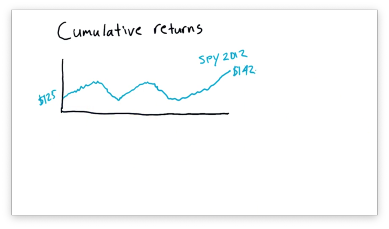
This stock started 2012 at $125 and finished at $142. However, when we hear about a stock on the news, we don't usually hear beginning and end prices, but rather something like: "SPY gained 13.6% in 2012."

That 13.6% is the cumulative return for SPY in 2012. In other words, the cumulative return for a stock is the total return for the stock over a given range.

We can calculate a cumulative return on a day t with a simple equation:

(price[t] / price [0]) - 1

If we set t equal to the last day in 2012, we can calculate the cumulative return as:

142 / 125 - 1 # = 1.136 - 1 = 13.6%

We can calculate and chart cumulative returns for the entire time period, just like we did with other statistics, such as the rolling mean.

Note that the shape of this chart is identical to the price chart but just normalized. In fact, the expression for cumulative return is identical to the expression for normalization we saw in a previous lecture.

Machine Learning Trading