How Machine Learning is Used at a Hedge Fund

The ML Problem

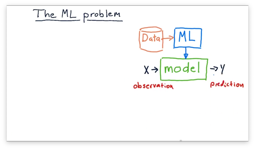
In most cases, we use machine learning algorithms to build a model. A model is essentially a function: it receives an input $X$ and produces an output $Y$.

Typically, $X$ is a measurement or set of measurements that we have taken or observed. The model processes $X$ and produces the output $Y$, which is usually a prediction about the world. For example, $X$ might be the current price of a stock, and $Y$ might be the future price of that stock.

$X$ can also be multidimensional; in other words, we might have a model that considers multiple features at once. For example, $X$ might be an array containing the current price, P/E ratio, and Bollinger bands for a stock. $Y$ is typically a single value and represents the one-dimensional prediction that we are trying to make.

Of course, there are many models that people have built that don't use machine learning at all, such as the Black Scholes model that predicts options prices. Models like these are mathematical models, which are derived analytically.

Machine learning models are different. The machine learning process involves running historical data through a machine-learning algorithm to derive a model based on that data. Later, when we need to use the model, we pass in new examples and receive fresh predictions.

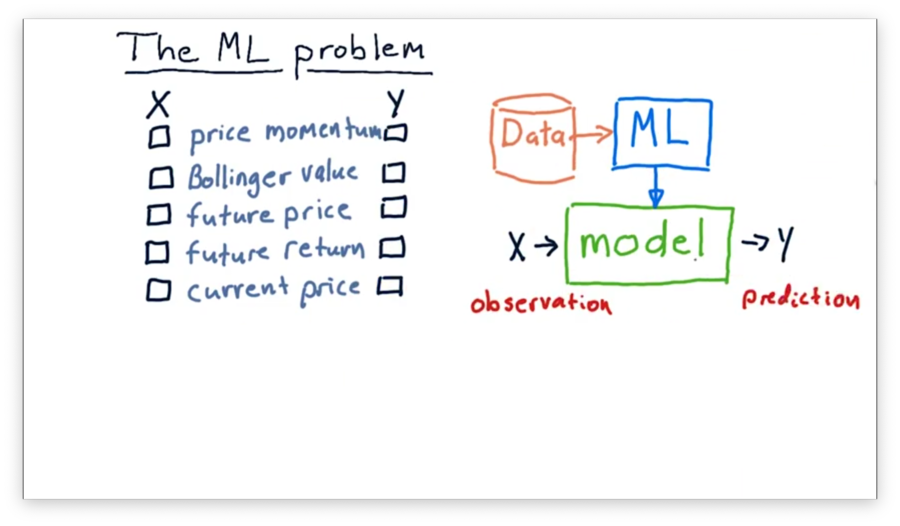
What's X and Y Quiz

Let's think about building a model to use in trading. Which of the following factors might be input values ($X$) to the model, and which might be output values ($Y$)?

What's X and Y Quiz Solution

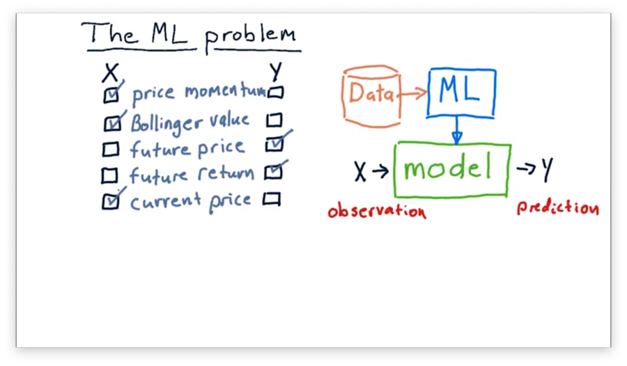
Since we often use models to predict values in the future, both future price and future return make sense as output values. Our model might make these predictions by considering price momentum, current price, and Bollinger values as input.

Supervised Regression Learning

The particular flavor of machine learning that we are going to focus on right now is called supervised regression learning. Let's break down each of these terms.

When we talk about regression, we are talking about making a numerical approximation or prediction. For example, predicting stock prices is a regression problem. Regression learning sits in contrast to classification learning, which involves classifying an object into one of several types.

In supervised learning, we present the algorithm with the correct answers during the training period. In other words, we show the machine an $X$ value and its corresponding $Y$ value. After seeing a sufficient number of input/output pairs, the algorithm is ready to predict $Y$ values for new, previously unseen $X$ values.

Finally, when we talk about learning, we are talking about training with data. In this class, for example, we are often taking historical stock data and training the system to predict the future price of the stock. We "teach" the algorithm to make new predictions by showing it relevant data from the past.

Many different algorithms use supervised regression learning techniques, and we can discuss four briefly here: linear regression, K-nearest neighbor, decision trees, and decision forests.

Linear regression involves finding the coefficients of a line that best fits the data. The coefficients are the parameters of the model, and linear regression is known as a type of parametric learning.

K-nearest neighbors (KNN) is another popular approach that evaluates an incoming $X$ by examining the K-nearest $(X, Y)$ pairs. Since this algorithm compares incoming data to instances of already-seen data points, this approach is known as instance-based learning.

Decision trees redirect incoming $X$ values down individual branches based on evaluations of factors of $X$ that occur at each node. The regression values are stored in the leaves of the tree, and the output of a decision tree for a given $X$ is the leaf in which the $X$ ends up.

Decision forests are composed of many decision trees queried in turn and combined in some way to provide an overall result.

Robot Navigation Example

Note: There is no write-up for this video. Honestly, this robot navigation example runs pretty far afield of the core course content. If you are really invested, watch the full video here

How it Works with Stock Data

Let's consider how we can generate the type of data we can feed into a machine learning algorithm in order to build a model.

Assume we have a pandas DataFrame containing historical features of a particular stock, arranged in the usual way: one row for each date with columns representing each metric.

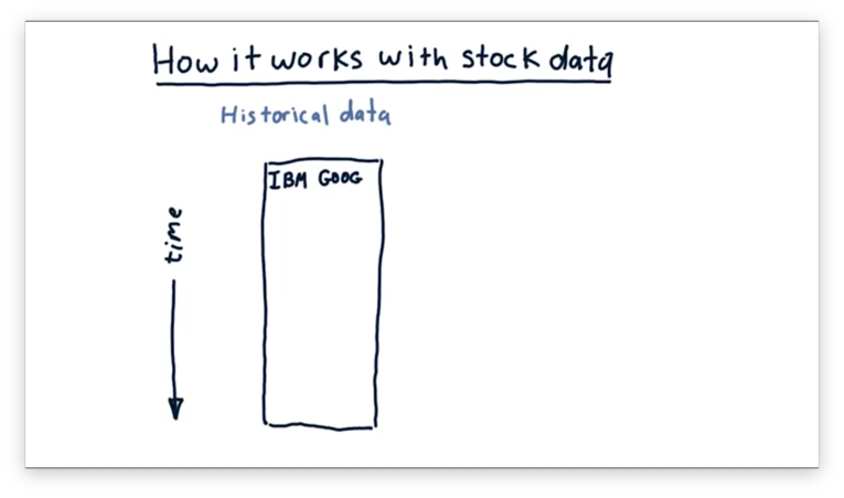
We might have many features for each stock, such as Bollinger Bands, momentum, and P/E ratio. We can represent each feature in a DataFrame, and then "stack" the DataFrames one behind the other.

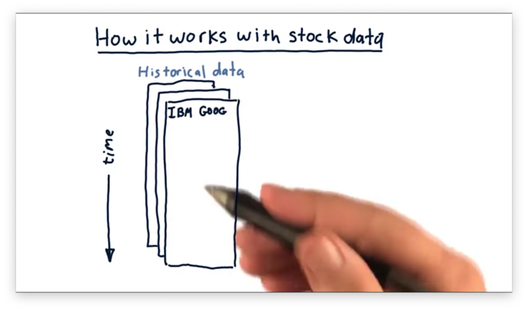
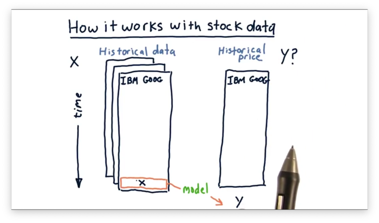
These features make up the input values - the $X$ - for the model that the machine learning algorithm synthesizes. In most cases, we want to use our model to produce a future price - the $Y$ - given this historical feature data as input.

To generate the model, we need to supply the machine learning algorithm with training examples containing stock features and the corresponding future price. Since we don't have prices in the future, we have to use historical prices.

Let's see how we can generate these examples starting from the first date d for which we have data. We can look at the stock features for d, and the price at some future date, such as d + 5. Note that even though the price is historical, it's in the future relative to d.

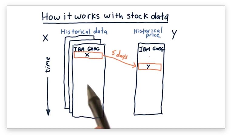
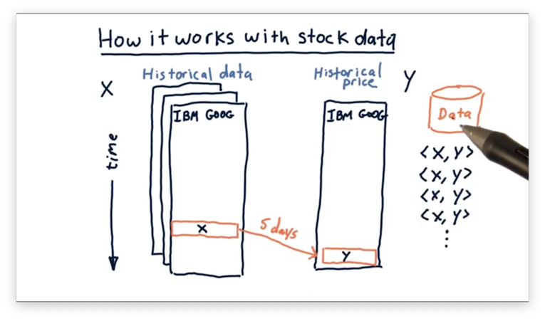
This pairing between features $X$ at d and future price $Y$ at d + 5 comprises our first training example. We can step forward day-by-day to generate subsequent examples mapping $X$ at d + n to $Y$ at d + 5 + n. Once this process is complete, we will have a large set of examples that we can use to build our model.

Example at a FinTech Company

We can use this process to build a machine-learning-based forecaster at a FinTech company.

The first step is to select which factors we think are essential in the forecast we want to generate. These factors - Bollinger Bands, P/E ratio, and others - are our $X$ values. They are measurable quantities about a company that can be predictive of its stock price.

The next step is to select the $Y$ that we want to predict. Usually, we want to predict a change in price or the future price of a stock.

Now that we know our $X$ and $Y$, we need to consider the scope of data we are going to use to train our system. For example, we need to select the range of dates we want to consider, be it three months, three years, or three decades. Additionally, we need to consider which symbols from the stock universe we want to include in training.

We can then select our historical $X$ and $Y$ values, scoped by the constraints we've outlined, to create the data that we use to train the model.

Next, we pass this data to our machine learning algorithm - KNN, linear regression, decision trees, or something else - and the algorithm converts the data into a model.

Once we have the model, we are ready to use it to generate predictions. We measure the pertinent features of the stock we are interested in and plug them into the model, which outputs the prediction.

Price Forecasting Demo

Note: There is no write-up for this video. Transcribing a walkthrough of some proprietary application that you and I are never going to use is pointless. If you are really interested, watch the full video here.

Backtesting

Once we have our model, we might start to get curious about the accuracy of the forecasts it provides and whether we can act on them.

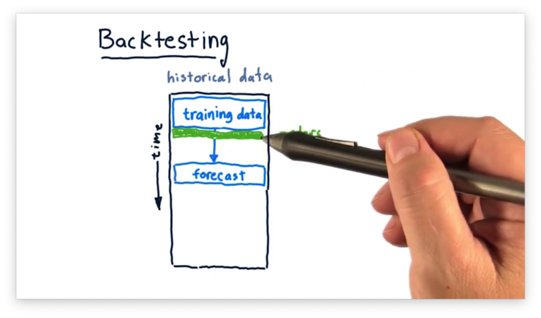
We can evaluate the performance of our model through backtesting. Backtesting is the process of applying a trading strategy or analytical method to historical data to see how accurately the strategy or method would have predicted actual results.

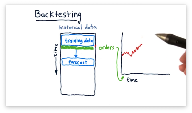
First, we limit our data to some subset and train a model on just that data. Next, we ask the model for a forecast of some time in the simulated future. Third, we place orders on the basis that the forecast is accurate, shorting or longing stocks as appropriate.

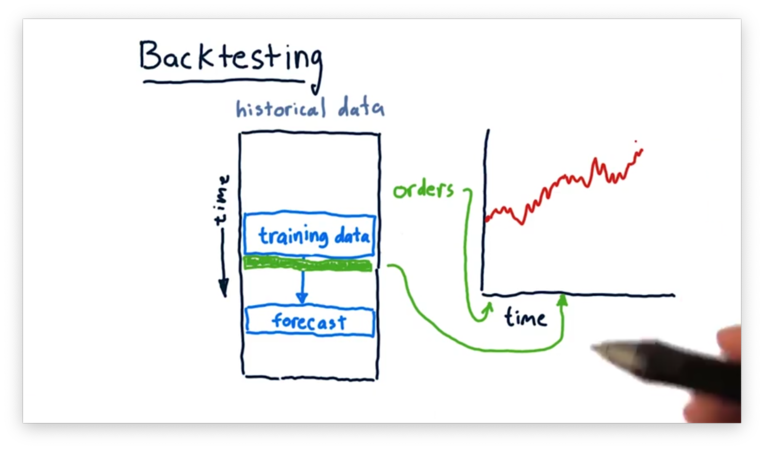
We can then roll time forward and see how the performance of our portfolio - measured by Sharpe ratio, daily return, or something similar - changes as the forecast does or does not come to fruition.

Finally, we repeat this process. We train a model based on a more recent subset of the data, make a prediction, and plot performance based on orders made in line with the prediction.

We can backtest our strategy against historical data to simulate the performance of our portfolio according to the strategy. Ultimately, the performance informs us whether the strategy is worth adopting.

ML Tool in Use

Note: There is no write-up for this video. Transcribing a walkthrough of some proprietary application that you and I are never going to use is pointless. If you are really interested, watch the full video here.

Problems With Regression

Regression-based forecasting is not without its issues. First, the forecasts we generate with this approach are often noisy and uncertain. Second, it's hard to know how confident we should be in a forecast. Additionally, it's not clear how long to hold a position or how to allocate to a position that has arisen from a forecast.

We can use reinforcement learning to address some of these issues. In reinforcement learning, the system learns a policy that guides its actions. In our case, the policy informs the system of whether to buy or sell a stock.

Problems We Will Focus On

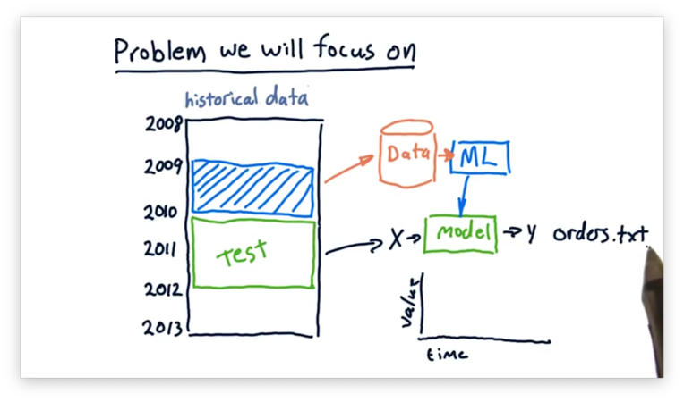
For the rest of this class, we are going to look at data from a specific period, train our models over that data, and then trade over some other period.

For example, we can use data from 2009 to train our models. Then, throughout 2010 and 2011, we can use our models to generate orders based on forecasts. As time passes, we can watch the performance of our portfolio change as the forecasts do or do not come true.