Machine Learning Trading
Reading and Plotting Stock Data
6 minute read
Notice a tyop typo? Please submit an issue or open a PR.
Reading and Plotting Stock Data
Data in CSV files
In this class, we work almost exclusively with data that comes from comma-separated values (CSV) files. As the name suggests, every data point in a CSV is separated by a comma.
Here is an example of a CSV that contains data related to weather conditions.
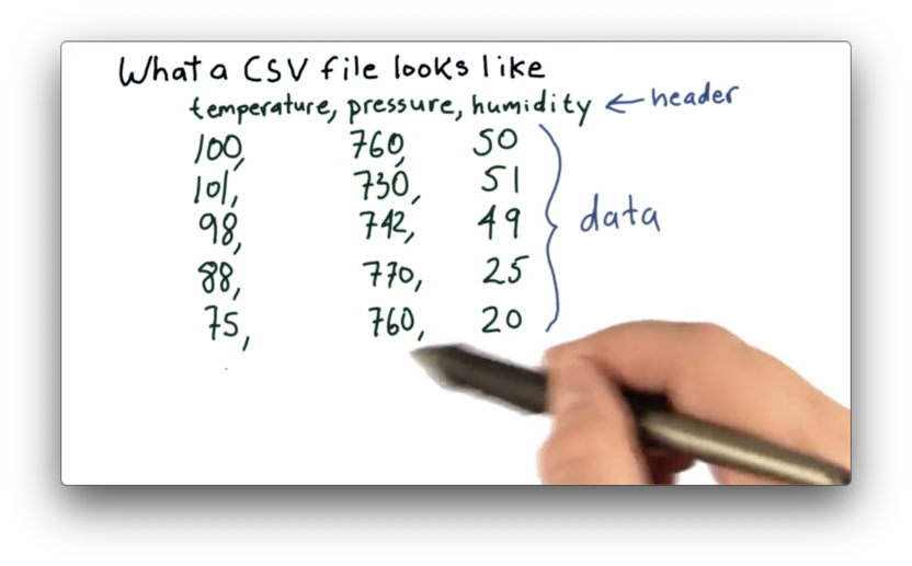
Most CSV files start with a header line, which describes the data present in the file. In this example, the header line is:
temperature,pressure,humidityThis header tells us that we have data points corresponding to temperature, pressure, and humidity.
Following the header line, we have several rows of data. Each row contains data points, separated by commas, corresponding to the values in the header. For example, the first row lists a temperature of 100, a pressure of 760, and a humidity of 50.
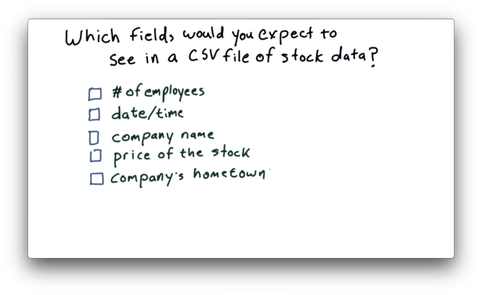
Which Fields Should Be In A CSV File Quiz
Which Fields Should Be In A CSV File Quiz Solution
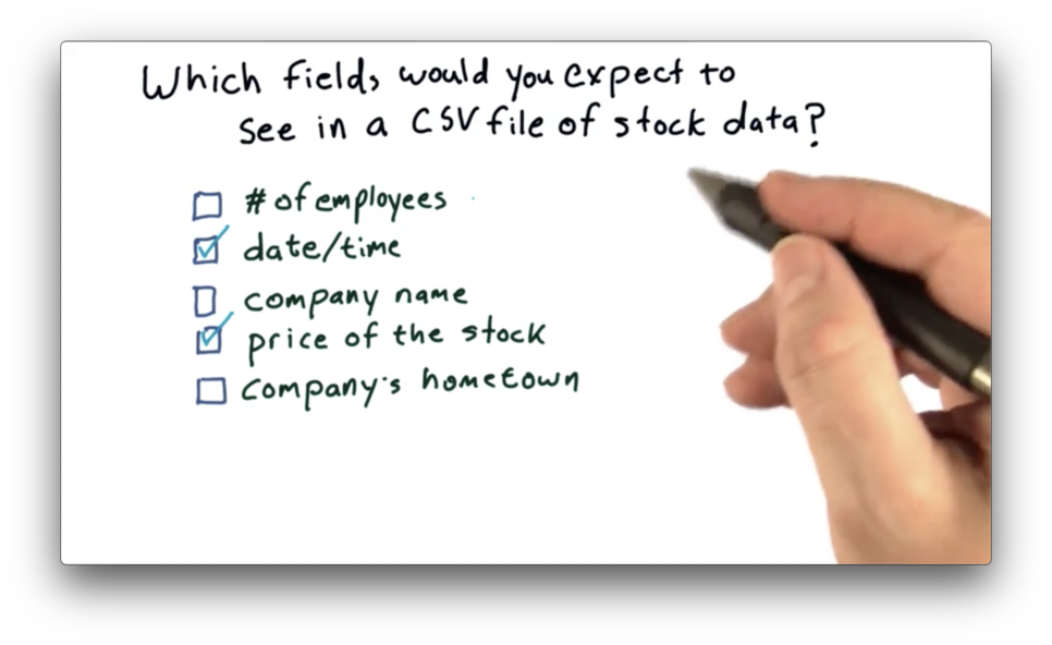
We want to include data that changes frequently; otherwise, we are wasting space including redundant data. Of the options given, both "date/time" and "price of the stock" are good fits. The other data points are either static or change relatively infrequently.
Real Stock Data
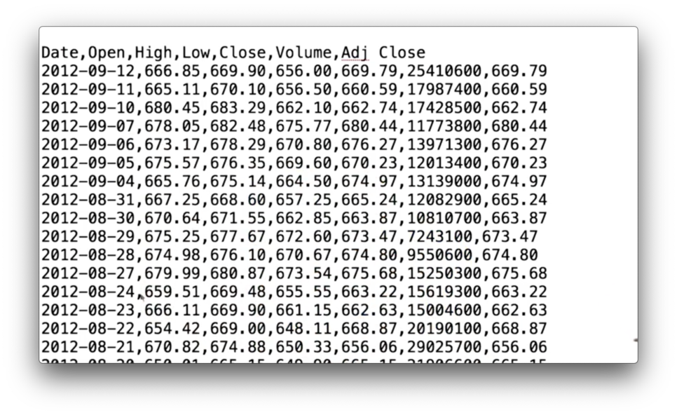
Let's take a look at real stock data, presented in the following CSV.
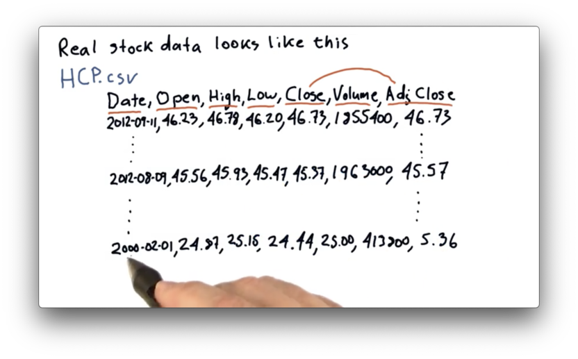
As always, we have a header row, which describes the columns in our data set.
The Date column refers to the date the data was captured. The Open column refers to the first price of the day for the stock. High and Low refer to the highest and lowest price the stock reached during the day, respectively. When the market closes, the last price recorded is the Close price. Finally, the number of shares traded is captured in the Volume column.
The adjusted close is a number that the data provider - Yahoo, in this case - calculates after considering stock splits and dividend payments. The Adj. Close column reflects this value.
Today (imagining we are in late 2012), the adjusted close and the close are the same. Naturally, no splits or dividends occurred between 4 P.M. and now. As we go back in time, however, we begin to encounter these events, and the close and adjusted close values correspondingly diverge.
If we look back to the first trading day in 2000, we see a close of $25.00 and an adjusted close of $5.36. The most recent close we see is $46.73.
If we compare just the closing prices, it seems like an investment in 2000 would have grown by less than 100%. If we instead compare the adjusted closes, the same investment would have grown almost 800%. The adjusted close allows us to incorporate events like splits and dividends into our ROI calculations.
Pandas DataFrame
In this course, we make heavy use of a python library called pandas, created by Wes McKinney. Pandas is used widely at hedge funds and by many different types of financial professionals.
One of the key components of pandas is the DataFrame. Here is a representation of a DataFrame containing closing prices.
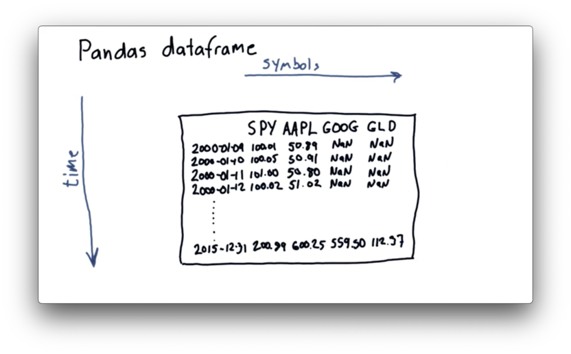
Across the top are the columns, and each column holds the symbol of a tradable entity, such as SPY (an ETF representing the S&P 500), AAPL (Apple), GOOG (Google), and GLD (a precious metals ETF). There is one row for each tradable day between 2000 and 2015.
The NaN values stand for "Not a Number", which pandas can use as a placeholder in the absence of meaningful data. We see NaN values for GOOG and GLD because neither existed as a publicly-traded entity in early 2000.
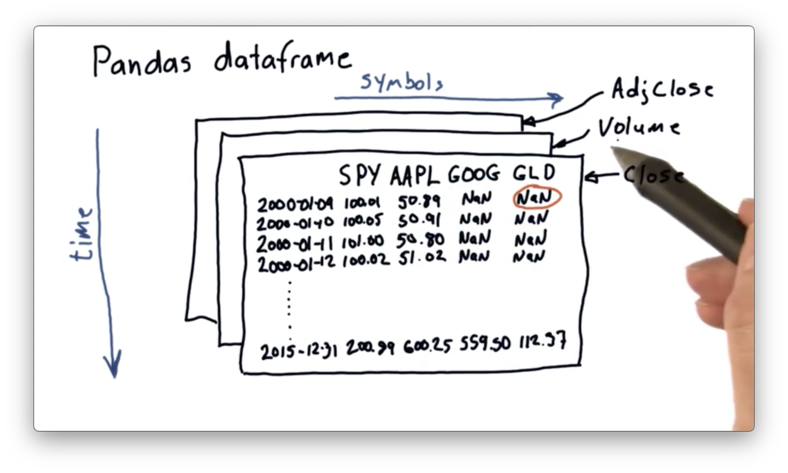
Pandas can also handle three-dimensional data. For example, we can build multiple DataFrames for the same symbols and dates, where each DataFrame contains information related to a different data point, such as close, volume, and adjusted close.
Example CSV File
Read CSV
Pandas provides several functions that make it easy to read in data like the CSV we just saw. The following code reads in the data from a file data/AAPL.csv into a DataFrame df:
import pandas as pd

df = pd.read_csv("data/AAPL.csv")
Note that we import pandas as pd to avoid having to write out the full pandas every time we want to call a method.
We can think of df as a 2D array that takes roughly the same shape as the CSV we see above, and if we print it out - print df - we see the following.
Printing an entire DataFrame is unwieldy, especially as our DataFrames grow in size, so we can use the following code to print out just the first five rows of the df:
print df.head()If we execute this code, we see the following.
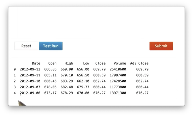
In addition to the named columns that we see in the CSV, we also see an unnamed column containing the values 0, 1, 2, 3, 4. This column is the index for the DataFrame, which we can use to access rows.
Similarly, we can use the following code to see the last five rows of df:
print df.tail()Documentation
Select Rows
Of course, we would like to be able to access more than just the first five or last five rows of our DataFrame. For more flexible row accesses, we need to look at slicing.
The following code demonstrates how to print the tenth through the twentieth rows of df:
print df[10:21]This code generates the following output.
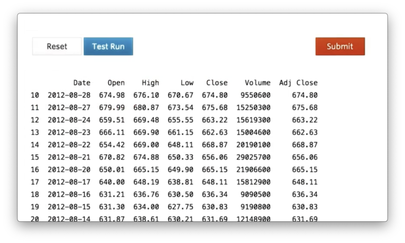
Generally, if we want to access rows n through m in df, we use the following syntax:
df[n:m + 1]Note that the range is upper-bound exclusive, which means it won't include the m-th row by default. Thus, we must slice up to, but not including, m + 1.
Documentation
Compute Max Closing Price
Let's assume we have a DataFrame df containing columns such as "Open", "High", "Low" and "Close", among others. If we'd like to retrieve just the "Close" column from df, we can use the following code:
close = df['Close']Given this object (technically a pandas Series), we can find the maximum value with the following code:
close.max()Documentation
Compute Mean Volume Quiz
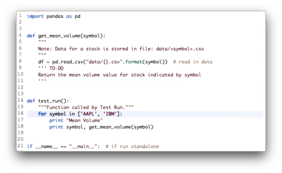
Your task is to calculate the mean volume for each of the given symbols.
Compute Mean Volume Quiz Solution
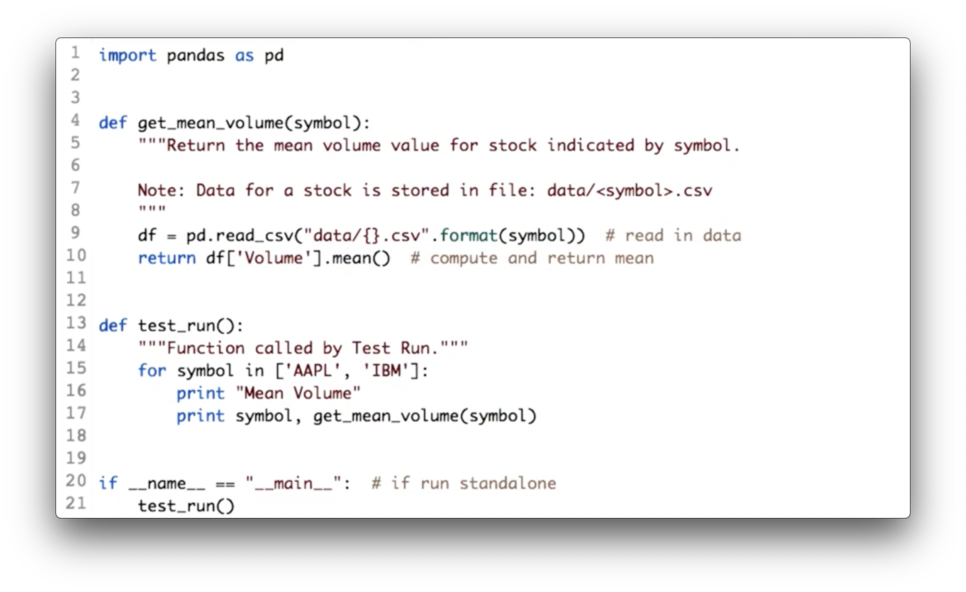
Given a DataFrame df containing a "Volume" column, the following code returns the mean of the values in that column.
df['Volume'].mean()Documentation
Plotting Stock Price Data
It's easy to plot data in a DataFrame.
First, we need a library called matplotlib. To plot the adjusted close of df, we can run the following code:
import matplotlib.pyplot as plt

df['Adj Close'].plot()
plt.show()
The generated plot looks like this.
Note how simple this graph is: there is no x-axis label, no y-axis label, no legend, and no title.
Documentation
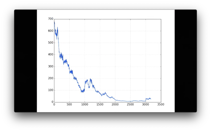
Plot High Prices for IBM Quiz
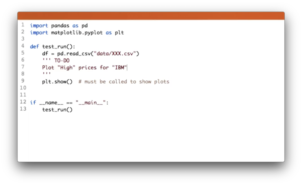
Your task is to plot the high prices for IBM.
Plot High Prices for IBM Quiz Solution
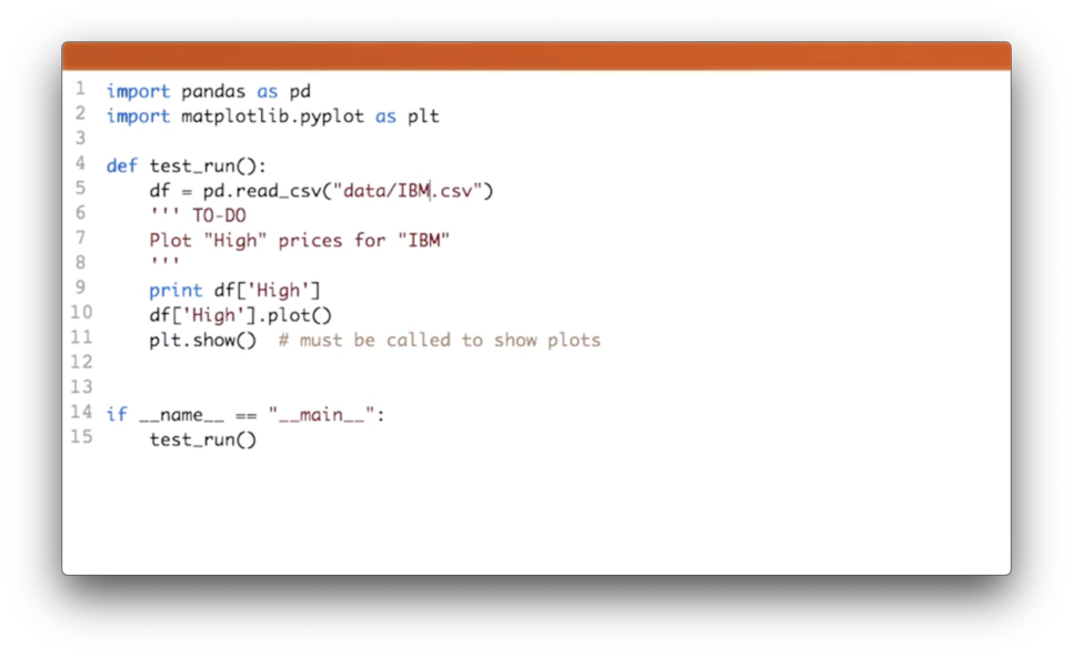
First, we need to make sure that we read in the right CSV, which we can accomplish with:
df = pd.read_csv('data/IBM.csv')Next, we can retrieve the "High" column and plot it:
df['High'].plot()Plot Two Columns
We don't have to plot only one column at a time. We can plot both the adjusted close and close of df with the following code:
df[['Close', 'Adj Close']].plot()
plt.show()
Here is the resulting graph.
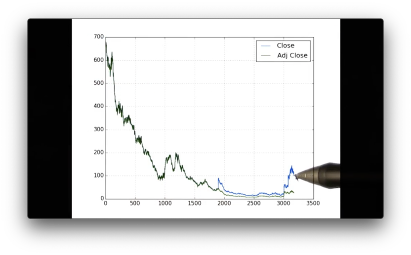
We can see the blue line, which corresponds to 'Close', and the green line, which corresponds to 'Adj Close'. Note that we didn't have to write any extra code to get these colors or the legend.
OMSCS Notes is made with in NYC by Matt Schlenker.
Copyright © 2019-2023. All rights reserved.
privacy policy