Machine Learning Trading
Sharpe Ratio and Other Portfolio Statistics
9 minute read
Notice a tyop typo? Please submit an issue or open a PR.
Sharpe Ratio and Other Portfolio Statistics
Daily Portfolio Values
We want to understand how to calculate the overall daily value of a portfolio so that we can compute statistics on portfolio performance.
Let's consider the following portfolio. Assume we start with a portfolio value of $1 million, and we track the portfolio from the beginning of 2009 to the end of 2011.
At the beginning of 2009, we split our $1 million into the following four allocations: 40% SPY, 40% XOM, 10% GOOG, and 10% GLD. We hold these positions for the entire 3-year period and assess whether we gained our lost money at the end of 2011.
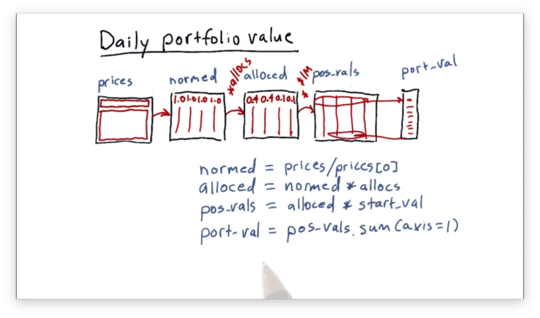
Let's look at how we can calculate the value of the portfolio day-by-day. We start with our prices DataFrame prices that contains columns for each of the four stocks, indexed by date.
First, we create a DataFrame normed that contains the normalized values of the prices in prices:
normed = prices / prices[0].valuesNote that the first row of normed contains all ones, and each subsequent row contains the ratio of the price on that day to the price on day one.
Next, we create a DataFrame alloced that multiplies the normalized prices for each stock by their corresponding allocation. Given an array of allocs - [0.4, 0.4, 0.1, 0.1] - we can create alloced like so:
alloced = normed * allocsNote that the first row of alloced contains the values of allocs, and each subsequent row contains the normalized price for each stock scaled by the corresponding allocations.
Our third step is to create a DataFrame pos_vals that holds the actual monetary value of our positions in each of the four stocks throughout time:
pos_vals = alloced * start_val # 1_000_000The first row of pos_vals gives us the initial amount of cash allocated to each stock - $400,000, $400,000, $100,000, and $100,000 - and each subsequent row adjusts that amount based on the normalized, allocation-scaled price value for that row.
In other words, each cell in pos_vals tells us how much our position in that stock is worth on that day.
Next, we can create a one column DataFrame port_val that condenses our individual position into one number reflecting the total value of the portfolio each day:
port_val = pos_vals.sum(axis=1) # Sum across columnsThe first row of port_val is simply the sum of the initial allocations: $1 million. Each subsequent row reflects the new value of the portfolio as the value of our positions changes as a result of stock price movement.
Portfolio Statistics
Now that we have port_val, the DataFrame containing the total daily value of the portfolio, we can compute several important statistics on the portfolio. These statistics allow us to assess the performance of the portfolio and the investment style of the portfolio manager.
For example, we can calculate daily returns, which gives us a measure of how our portfolio performed on a given day relative to the previous day.
We can construct a DataFrame daily_returns that contains the daily returns of our portfolio:
daily_returns = (port_val / port_val.shift(1)) - 1
daily_returns.iloc[0] = 0
Whenever we calculate daily returns, the first value is always going to be zero because there is no previous day for comparison. We want to exclude this first entry from any calculations that we do over daily returns.
daily_returns = daily_returns[1: ]Now that we have this information, we can compute four critical statistics regarding the performance of a portfolio: cumulative return, average daily return, standard deviation of daily return, and Sharpe ratio.
Cumulative return is a measure of how much the value of the portfolio has changed from beginning to end. We can calculate the cumulative return like so:
(port_val[-1] / port_val[0]) - 1The average daily return is simply the average of the values in daily_returns:
daily_returns.mean()We can calculate the standard deviation of the values in daily_returns similarly:
daily_returns.std()The Sharpe ratio is a bit more complicated, so we will spend some more time talking about it next.
Which Portfolio is Better Quiz
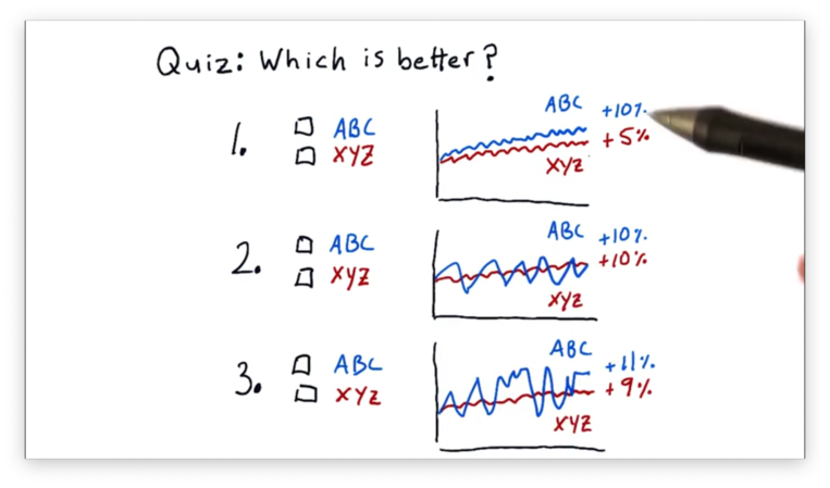
The Sharpe ratio allows us to consider our returns in the context of risk: the standard deviation, or volatility, of the returns. When we look at portfolio performance, we don't typically look at raw returns; instead, we adjust the returns received for the risk borne.
With this in mind, let's look at three comparisons of two stocks, ABC and XYZ, and decide which is better.
Which Portfolio is Better Quiz Solution
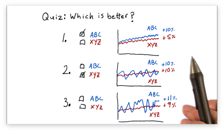
For the first comparison, ABC is better. ABC and XYZ have similar amounts of volatility, but ABC has double the return of XYZ.
For the second comparison, XYZ is better. Both ABC and XYZ have the same return, but ABC is much more volatile than XYZ.
For the third comparison, we can't tell which is better, given the information provided. ABC has a higher return than XYZ, but that return is offset by higher volatility.
We need a qualitative measure to compare ABC and XYZ in this third example, and the Sharpe ratio is that measure.
Sharpe Ratio
The Sharpe ratio, named for William Sharpe, is a metric that adjusts return for risk, and it enables us, quantitatively, to assess and compare the portfolios from the quiz above.
We would assume that all else being equal, lower risk is better, and higher return is better. Indeed, the Sharpe ratio validates these assumptions.
It's always possible that the performance of an asset is less than the risk-free rate of return: the interest rate our money would receive if we just put it in a risk-free asset like a bank account. The Sharpe ratio accounts for this possibility by including the risk-free rate of return in its calculation.
Lately, however, the risk-free rate of return is about 0. If you were to put your money in the bank or buy very short-term treasury bonds, you'd receive virtually no interest.
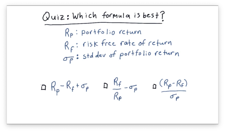
Form of the Sharpe Ratio Quiz
Consider the following three factors.
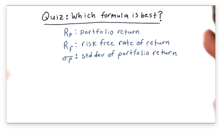
How would you combine these three factors into a simple equation to create a metric that provides a measure of risk-adjusted return?
Form of the Sharpe Ratio Quiz Solution
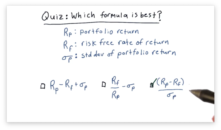
Only the third choice meets the two criteria we described earlier; all else being equal, higher returns increase our metric, and lower risk increases our metric. Additionally, a higher rate of risk-free return decreases our metric.
Computing Sharpe Ratio
Given a daily portfolio return and a daily risk-free rate of return , we can formulate the Sharpe ratio as:
That is, the Sharpe ratio is the expected value of the difference of the portfolio return and the risk-free rate of return divided by the standard deviation of that same difference.
When we talk about expected value, we are talking about expectations of events that occur in the future. This forward-looking formulation of the Sharpe ratio is called the ex-ante formulation.
Of course, to calculate the expected value going forward, we have to look back at the historical values. We can use the historical mean of the differences between and as the expected value going forward.
What is the risk-free rate? One value often used is the London Inter-bank Offered Rate. Another value used is the interest rate on a three-month treasury bill (T-bill). More recently, however, people have been using zero for the risk-free rate.
Does this mean that we need to retrieve the corresponding risk-free rate for each daily return we have? While LIBOR and the three-month T-bill interest rate do change slightly day-to-day, we don't actually need to record their daily values.
In fact, the risk-free rate is not usually given daily, but rather on an annual or six-month basis. With a little bit of math, we can convert that annualized rate into a daily rate.
Let's look at an example. Assume our risk-free rate is 10% per year, or 0.1. That means that if we start at the beginning of the year with a value of 1.0, we end the year with a value of 1.1.
We need to find a number that equals 1.1 when multiplied to our balance each day in the 252-day trading year. In other words,
Of course, is the multiple. The daily risk-free rate is , or 0.038%.
Note that this value is constant throughout the time period, and remember that the standard deviation of a set of numbers is unaffected if each number is shifted by the same amount. As a result, we can simplify our formula for the Sharpe ratio:
Since many people have been using zero recently for the risk-free rate of return, we are going to follow suit. Our final, simplified Sharpe ratio formula is:
But Wait, There's More!
The Sharpe ratio for the same asset can vary widely depending on how frequently we sample it. If we sample the prices every year and calculate the Sharpe ratio based on yearly statistics, you'll get one number. If we sample monthly or daily, we'll get different numbers.
The Sharpe ratio was initially envisioned as an annual measure. As a result, if we are sampling at nonannual frequencies, we need to incorporate an adjustment factor.
where
As an example, there are 252 trading days in a year, so if we are using daily data, then . If are taking weekly samples, then .
Note that is equal to the rate of sampling, not the number of samples we take. For instance, assume we are trading for 85 days. Because we are sampling at a daily rate, we set , not .
Bringing it all together, given a daily portfolio return and a daily risk-free rate of return , we can formulate the Sharpe ratio as:
What is the Sharpe Ratio Quiz
Assume we have been trading a strategy for 60 days now. On average, our strategy returns one-tenth of one percent per day. Our daily risk-free rate is two one-hundredths of a percent. The standard deviation of our daily return is one-tenth of one percent.
What is the Sharpe ratio of this strategy?
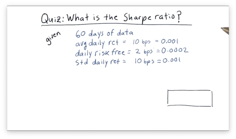
In financial terminology, one one-hundredth of one percent is known as a basis point, or "bip". Instead of saying, for example, that our strategy returns one-tenth of one percent per day, we could say it returns 10 bps per day.
What is the Sharpe Ratio Quiz Solution
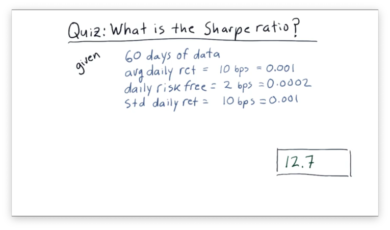
Let's recall our formula for the Sharpe ratio:
Given that on average, on average, and , with a daily sample rate:
OMSCS Notes is made with in NYC by Matt Schlenker.
Copyright © 2019-2023. All rights reserved.
privacy policy