Machine Learning Trading
How Hedge Funds Use the CAPM
10 minute read
Notice a tyop typo? Please submit an issue or open a PR.
How Hedge Funds Use the CAPM
Risks for Hedge Funds
A typical hedge fund develops methods to find performant stocks. The informational edge they are seeking is usually market-relative, meaning that they are looking for stocks that rise more than the market when the market goes up or stocks that fall less than the market when the market goes down. If the information they have is reliable, they can take advantage of the CAPM to virtually guarantee a positive return.
Two Stock Scenario
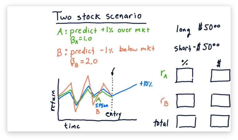
As an illustration of how hedge funds use CAPM, let's consider a two-stock scenario.
Suppose our hedge fund has done some research and they think that stock A is going to go up 1% over the market in the next 10 days; in other words, they are predicting an of 0.01 for stock A. As well, they have used historical pricing information to observe a of 1.0 for stock A.
Our hedge fund has also done some research on stock B, and they are predicting an value of -0.01 for this stock. Additionally, they have observed a historical of 2.0 for stock B.
We should long stock A and short stock B since we think the former is going to go up relative to the market, while the latter is going to go down. This type of long-short portfolio is widespread amongst hedge funds.
Consider the following scenario. Let's assume that the market stays flat, returning 0%, over the next 10 days and that we enter the following positions today: a $50 long position in stock A and a $50 short position in stock B. Let's also assume that our predictions are perfect. Stock A rises 1% above the market, and stock B falls 1% below the market.
Consider the returns of stock A, using the CAPM equation.
Since the market returned 0%, the equation simplifies.
Since is 0.01, our return is 1% of $50, or $0.50.
Now, consider the returns of stock B, using the CAPM equation.
Again, since the market returned 0%, the equation simplifies.
Since both and our investment in stock B are negative, we actually made a profit: -1% of -$50, or $0.50.
Altogether we made $1, a 1% return on our total investment.
Two Stock Scenario Quiz
Let's consider another scenario now.
Instead of staying flat, suppose that the market went up 10%. What are the relative and absolute returns for both stocks, and what is our total return, both relative and absolute?
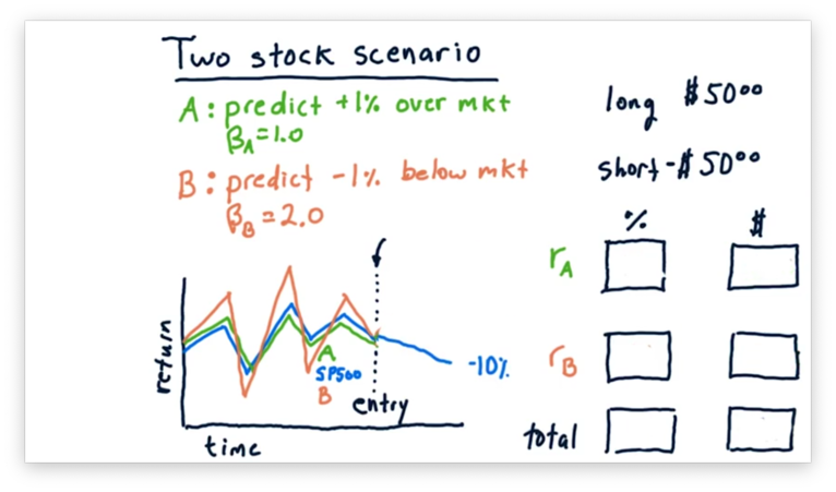
Let's also consider the scenario where the market goes down 10%. What are the relative and absolute returns for both stocks, and what is our total return, both relative and absolute?
Two Stock Scenario Quiz Solution
Let's first look at the case where the market rises by 10%.
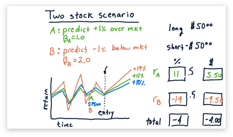
Consider stock A, which has a of 1.0 and an of 0.01. A of 1.0 tells us that for every percentage point that the market moves, stock A moves one percent. An of 0.01 tells us that stock A will move 1% above its movement with the market.
As a result, stock A moves 10% plus 1%, for a total relative return of 11%, and a total absolute return of $5.50, 11% on a $50 investment.
Let's consider stock B now, which has a of 2.0 and an of -0.01. A of 2.0 tells us that for every percentage point the market moves, stock A moves two percent. An of -0.01 tells us that stock B will move 1% below its movement with the market.
As a result, stock B moves 20% minus 1%, for a total relative return of 19%. However, since we shorted stock B, this return is actually -19%, and we have lost $9.50.
Let's compute the total return. Since we gained $5.50 on stock A and lost $9.50 on stock B, our total absolute return is -$4.
Calculating the relative return is a little tricky; that is, we can't just add 11% and -19% to get -8%. Instead, since we split our investment across stock A and stock B, our actual return is one-half of 11% plus one-half of -19%, or -4%.
Now, let's look at the case where the market falls 10%.
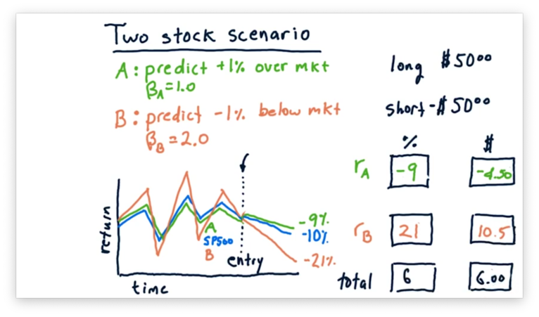
In this case, stock A falls with the market, but does 1% better, for a total relative loss of 9%, which equates to a $4.50 loss on a $50 investment.
Stock B falls twice as hard as the market, and does 1% worse on top of that, for a total relative loss of 21%. However, since we shorted stock B, this loss is actually a 21% gain, or a gain of $10.50 on a $50 investment.
Overall, this market scenario nets us 6%, or $6 on a $100 investment.
Two Stock CAPM Math
Recall how we use the CAPM to represent the return, , for our overall portfolio. For each individual stock, , we compute return, , as the product of and the return on the market, , plus . The value of is the sum of each multiplied by its corresponding weight, .
Let's expand this sum, considering our two stocks, A and B, from before.
Stock A has a of 1.0 and an of 0.01. Stock B has a of 2.0 and an of -0.01. Our portfolio has a 50% investment in stock A and a -50% investment in stock B. Let's plug these values into the CAPM equation.
Using the CAPM, we have determined that our expected return for this portfolio is equal to 1% minus one-half of the market return.
We can double-check this result by plugging in the market return from one of our previous examples. Let's look at the case where the market went up 10%.
Remember how we arrived at the 1% portfolio . We researched the stocks that we selected for our portfolio and found information that led us to believe that one would outperform the market by 1% and that the other would underperform the market by 1%.
On the other hand, we don't have any knowledge about what is going to happen in the market overall; that is, we have no control over the component of CAPM that incorporates market return. If we can eliminate this component, we can guarantee our 1% return, regardless of market movement.
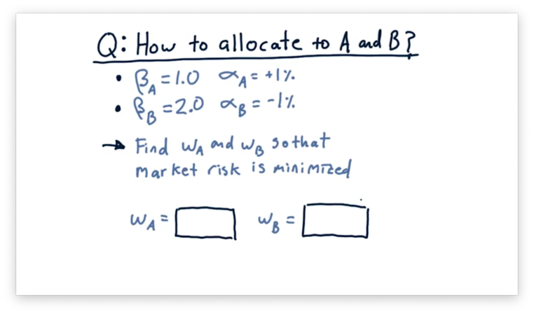
We can eliminate market risk by making . Since we can't change the individual and values to make this happen, we need to adjust our allocations instead. Essentially, we need to solve the following equation for and .
Allocations Remove Market Risk Quiz
Let's look at our two stocks again. Stock A has a of 1.0 and an of 0.01. Stock B has a of 2.0 and an of -0.01. What should the weights be for stock A and stock B so that we can minimize market risk?
Allocations Remove Market Risk Quiz Solution
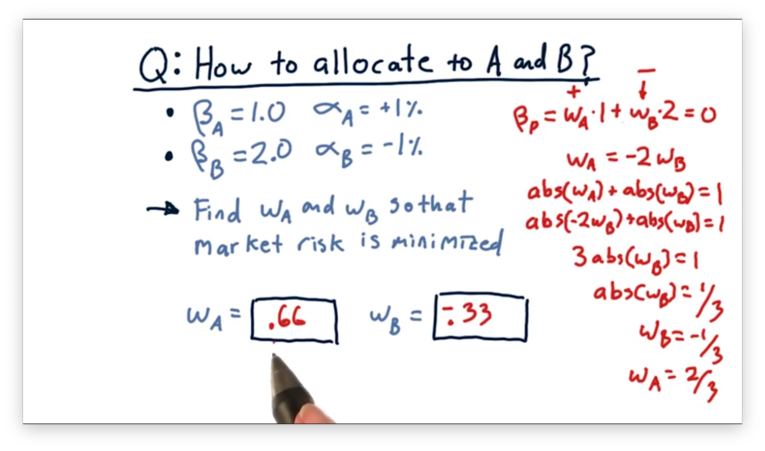
We need to solve the following equation.
We also know that the sum of the absolute values and should equal one.
If we substitute for , we can solve for .
However, since we want to short B, is actually , not . We can now solve for .
If we plug these two weights back into our original equation, we can verify that we do get an overall of 0.
How Does It Work
Now that we have calculated weights for stock A and stock B that eliminate market risk let's see how they work using the market conditions we have been examining.
Let's look at the scenario where the market goes up 10%. Using weights and , we can use the CAPM to compute portfolio return.
Because of the work we have already done, we know that the sum of the components that consider market return equals zero, so we can drop them from the equation.
Let's plug in the appropriate variables.
We can see that the expected return for our portfolio is 1%, irrespective of market movement.
We need to add some caveats here. Specifically, the values of and that we calculated using historical data are not guaranteed to carry into the future. This portfolio is not a guaranteed investment, by any means, but rather an example of how we can use long-short investing to reduce overall exposure to the market.
OMSCS Notes is made with in NYC by Matt Schlenker.
Copyright © 2019-2023. All rights reserved.
privacy policy