The Fundamental Law of Active Portfolio Management

Grinold's Fundamental Law

In the 1980s, Richard Grinold was seeking a method for relating three factors - performance, skill, and breadth - in investing.

On the one hand, an investor might see strong portfolio performance if they pick just one or two stocks that post fantastic returns. On the other hand, an investor might also see strong performance if they pick many stocks that each posts an average return. We can think of skill as the quality of each pick and breadth as the number of picks.

Grinold felt that there must be some equation whereby we could combine skill and breadth to create an estimate of performance. He developed a relationship called the fundamental law of active portfolio management, which relates performance, $P$, skill, $S$, and breadth, $B$, in the following equation.

We measure performance using a metric called the information ratio. The information ratio is very similar to the Sharpe ratio; however, the Sharpe ratio refers to risk-adjusted returns overall, and the information ratio refers to only the risk-adjusted returns that exceed the market or another portfolio benchmark.

We measure skill using a metric called the information coefficient. Breadth simply refers to the number of trading opportunities that we take.

Notice what this relationship is saying: we can improve the performance of our portfolio by either improving our skill in selecting stocks or by investing in more stocks.

The Coin Flipping Casino

Investing in a stock is, in some ways, similar to betting on a coin flip. In both cases, we make a decision and then earn or lose money based on that decision.

Let's run with the coin flip analogy and imagine that we are in a coin-flipping casino. We are going to make bets on coin flips, and if the coin comes up heads, we win; otherwise, we lose.

For a particular coin flip, we can place an even money bet of $N$ tokens. If we win - the coin comes up heads - we win $2N$ tokens. If the coin comes up tails, we lose all $N$ tokens.

At this casino, there are 1000 betting tables, each with their own coin. We have 1000 tokens, and we can choose to bet however we'd like; for example, we can bet 1 token on 1000 tables, 1000 tokens on 1 table, or something in the middle.

Once we have distributed our tokens - in other words, placed our bets - the coins are flipped all at once, and the winnings are paid out.

To make the analogy more realistic, let's assume that the coin is biased, and we know that it shows heads 51% of the time and tails 49% of the time. This informational edge is similar to the alpha value we associate with particular stocks that we think are going to outperform the market.

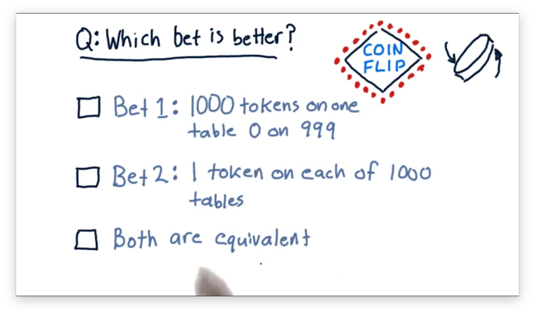
Which Bet is Better Quiz

Let's consider two different ways to bet.

One approach is to put all 1000 tokens on one table and zero tokens on the other 999 tables. Another approach is to put one coin on each of the 1000 tables. Which of these approaches is better, or is it the case that they are equivalent?

Which Bet is Better Quiz Solution

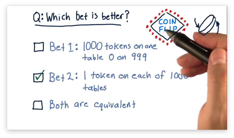
The first bet is very risky; that is, there is a 49% chance that we are going to lose all of our money with the single flip of a coin. The second bet is much less risky. By distributing our tokens across all one thousand tables, we only lose all of our money if we lose all 1000 bets: a very low probability indeed.

Since the expected return for each of these bets is the same, the second bet is a better choice from the perspective of risk-adjusted reward.

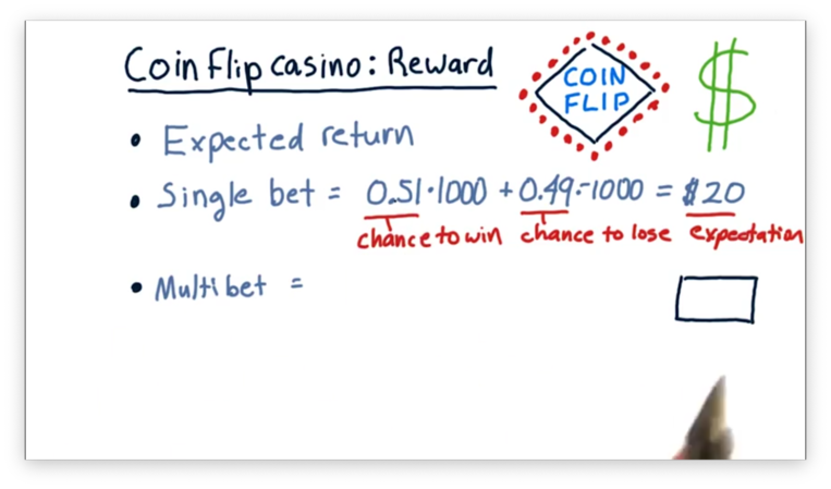
Coin-Flip Casino: Reward Quiz

To figure out which of these different scenarios is best, we need to consider reward and risk. When we talk about reward in this situation, we are talking about expected return.

In the single-bet case, where we bet 1000 chips at once, our expected return is the chance of winning the bet times the amount that we would win plus the chance of losing the bet times the amount that we would lose.

Since we are using a biased coin, we have a 51% chance of winning 1000 tokens and a 49% chance of losing 1000 tokens. If we multiply this out, we see that our expected return is 20 tokens.

What is the expected return in the multi-bet case, where we bet 1000 tokens across 1000 different tables?

Coin-Flip Casino: Reward Quiz Solution

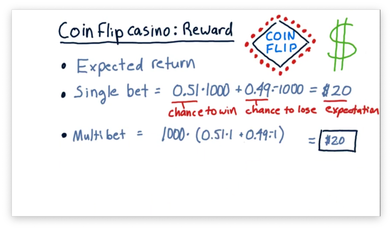
In this case, we have the same chances of winning and losing - 51% and 49%, respectively - but the amount we stand to win or lose on any bet is only one dollar. Since we are placing 1000 bets, our overall expected value is 1000 times the expected value of any individual bet.

Notice that for both the single-bet and multi-bet scenarios, the expected return - the reward - is precisely the same. To understand why the multi-bet setup is a better choice, we have to also consider the risk inherent in each scenario.

Coin-Flip Casino: Risk 1

There are several ways that we might consider risk in this scenario.

First, let's look at the chance of us "losing it all". In other words, after we have placed our bets, what is the chance that every coin flip we bet on lands on tails?

In the single-bet case, where we bet everything on a single table, and the outcome is determined by the flip of a single coin, there is a 49% chance we lose all of our money. That's a very high probability of loss; would you bet your savings account on odds like that?

Let's now consider the multi-bet scenario, where we bet a single token across 1000 tables, and our return is determined by the result of 1000 coin flips.

In this scenario, the chance that we lose all of our money is the chance that we lose the first flip times the chance that we lose the second flip - and so forth - times the chance that we lose the one-thousandth flip.

Formally, the chance of losing all of our money in the multi-bet scenario is $0.49^{1000}$, which is an infinitesimally small probability indeed.

Coin-Flip Casino: Risk 2

Another way we might examine risk in this experiment is to consider the standard deviation of all of the individual bet outcomes.

In the multi-bet scenario, we are going to have a collection of 1000 outcomes that are either 1 or -1. Either we won the bet and won a token, or we didn't and lost a token. The standard deviation for this case is 1.0.

In the single-bet scenario, we are going to have a collection of 999 outcomes that are exactly zero and one outcome that is either 1000 or -1000. Regardless of whether we win or lose, the standard deviation of outcomes in this scenario is 31.62.

Using this quantification of risk, we can see that the single-bet scenario is almost 32 times riskier than the multi-bet scenario.

Coin-Flip Casino: Reward/Risk Quiz

Now we can consider the risk-adjusted reward.

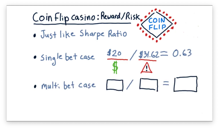
Let's look at the single-bet case first. In this case, the expected reward is $20, and the expected risk is $31.62. If we divide the reward by the risk, we get a value of 0.63.

What is the risk-adjusted reward calculation for the multi-bet case?

Coin-Flip Casino: Reward/Risk Quiz Solution

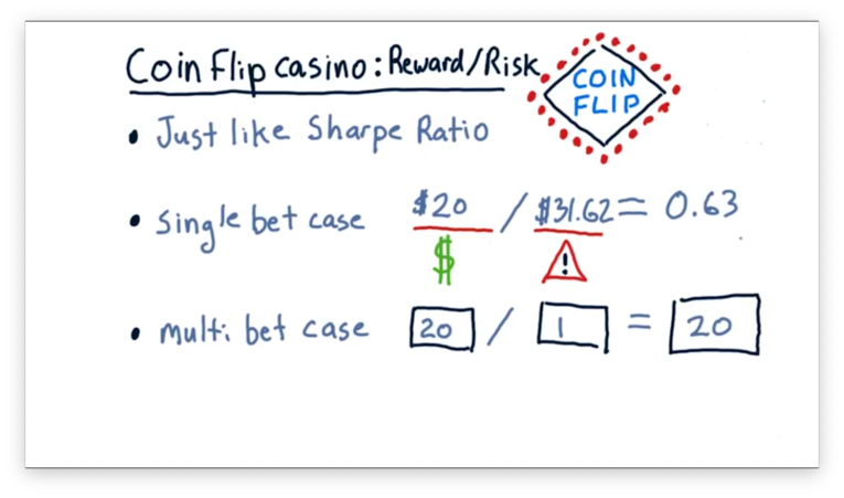
In the multi-bet case, the reward was the same - $20 - but the risk was much smaller: $1. Thus, the risk-adjusted reward for this scenario is 20, which is much higher than that of the single-bet scenario.

The take-home message here is that we can increase the risk-adjusted reward simply by spreading our money across a large number of bets.

Coin-Flip Casino: Observations

As we saw, the risk-adjusted reward for the single-bet case, $RAR_{single}$, is 0.63. Alternatively, the risk-adjusted reward for the 1000-bet case, $RAR_{multi}$, is 20. Notice the following relationship.

As we increase the number of bets that we place, the overall risk-adjusted reward increases with the square root of that number. Put another way, we can increase the overall risk-adjusted reward of our bets by improving the odds of a single bet or by spreading our money out over more bets.

This relationship is identical to the fundamental law of active portfolio management, which relates performance, skill, and breadth in the following way.

From this relationship, we can see that we can improve overall investment performance either by improving skill - how good we are at picking stocks - or by increasing the number of investment opportunities we take.

Coin-Flip Casino: Lessons

Consider now the results of this thought experiment. Our casino enabled us to allocate our 1000 tokens to 1000 tables. We looked at two extreme cases: one where we put a small bet on all 1000 tables and another where we put all our money on one table.

We saw that the expected return was the same in both cases - about $20 - but the risk was substantially higher for the single-bet case. This was true for the two types of risk we examined: risk of "losing it all" and risk as standard deviation.

When we consider risk and reward together, we come away with three lessons. First, a higher alpha generates a higher Sharpe ratio. Second, more execution opportunities provide a higher Sharpe ratio. Third, the Sharpe ratio grows as the square root of breadth.

Back to the Real World

Let's consider two real-world funds.

The first is Renaissance Technologies, a hedge fund founded by Jim Simons, a math and computer science professor. The second is Warren Buffett, the investor who runs Berkshire Hathaway.

Both of these funds have produced similar returns over the years, yet they have very different investment styles. On the one hand, Buffett holds about 120 stocks and doesn't trade them, while, on the other hand, Renaissance Technologies trades upwards of 100,000 times a day.

We can use the fundamental law of active portfolio management to understand how two funds can act so differently and yet post similar returns.

IR, IC and Breadth

Recall that we use the CAPM equation to determine the return on a portfolio, $r_p$, for a particular day, $t$. Given a portfolio beta, $\beta_p$, a portfolio alpha for $t$, $\alpha_p(t)$, and the market return for $t$, $r_m(t)$, then

We can break this equation into two main components: a market component comprising $\beta_pr_m(t)$, and a skill component consisting of $\alpha_p(t)$.

The information ratio is the Sharpe ratio of the observed $\alpha$ values for a portfolio over many periods. Since the alpha component quantifies returns exceeding the market, we can think of the information ratio as a measure of risk-adjusted excess return.

Formally, given a collection of $\alpha_p$ observations, $\Alpha$, we can calculate the information ratio of the portfolio, $IR_p$, as

We can derive the daily values of $\alpha_p$ by looking back at the daily portfolio returns and subtracting the market component, $\beta_pr_m(t)$.

Information ratio is valuable in many different situations, not just in the fundamental law of active portfolio management. For example, people frequently use information ratio as a measure of portfolio manager performance.

IR, IC and Breadth Continued

The information coefficient (IC) is the correlation of the manager's forecast to actual returns. IC can range from -1, a completely incorrect forecast, to 1, a perfectly correct forecast.

Breadth represents the number of trading opportunities an investor encounters per year. Warren Buffett holds 120 stocks, so he sees 120 trading opportunities per year. On the other hand, Jim Simons, who trades over 100,000 times a day, has a much larger breadth.

The Fundamental Law

Given an information coefficient, $IC$, and A breadth, $BR$, the fundamental law of active portfolio management states the following equation to calculate the information ratio, $IR$.

In other words, the performance of the fund is due to the stock-picking skill of the manager times the square root of the number of investments.

One consequence of this relationship is that while we might be very skilled at selecting stocks, we must have multiple trading opportunities available to us if we want to operationalize this skill.

If we want to improve the performance of our fund, we can either focus on improving our skill or increasing our breadth. Most investors find it very hard to improve their skill, so instead, they look to increase their breadth by finding additional equities or markets to analyze.

Simons vs. Buffet Quiz

How can we relate the performance of Renaissance Technologies - really, Jim Simons - and Warren Buffett?

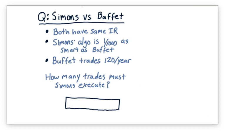
For this problem, let's assume that Simons and Buffett both have the same information ratio. Let's also assume that Simons's stock-picking algorithms are only about 1/1000th as smart as Buffett's; in other words, Simon's information coefficient is 1/1000th that of Buffett.

If Buffett trades 120 times a year, how many times must Simons trade to maintain the same information ratio as Buffett?

Simons vs. Buffet Quiz Solution

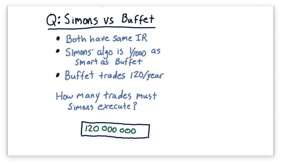
If Buffett trades only 120 times per year, Simons has to trade 120,000,000 times to match Buffett's performance.

Let's step through the math. Since Buffett and Simons both have the same information ratio, we can set the equation for $IR_B$ equal to the equation for $IR_S$.

Furthermore, we know that Simons's IC is 1/1000th Buffett's IC.

We can manipulate this equation to isolate $B_S$.

Since we know that $B_B = 120$, we can solve for $B_S$.