Machine Learning Trading
The Power of NumPy
14 minute read
Notice a tyop typo? Please submit an issue or open a PR.
The Power of NumPy
What is NumPy?
NumPy is a numerical library written in Python that focuses on matrix objects called ndarrays. NumPy delegates most of its core computation to underlying C and Fortran code, which means that NumPy is very fast. Indeed, many people use Python for financial research because of the functionality provided by NumPy.
Relationship to Pandas
Let's look back at our DataFrame df.
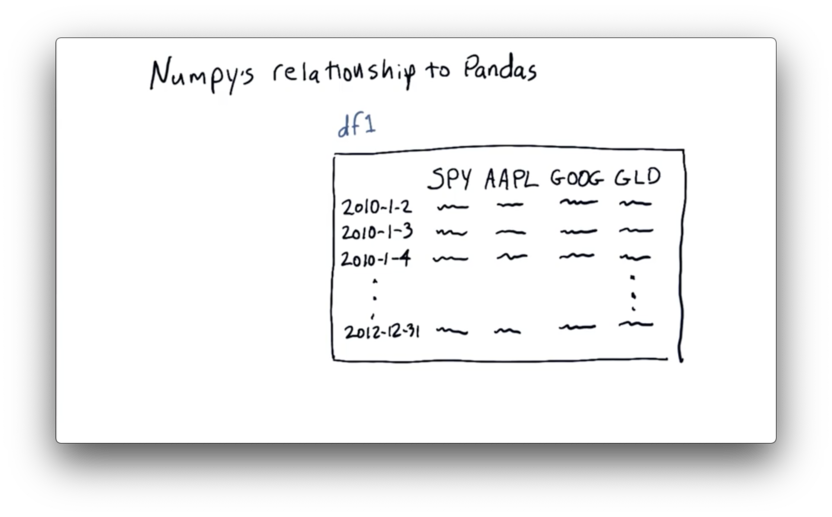
Just as NumPy is a wrapper around C and Fortran code, pandas is a wrapper of sorts around NumPy.
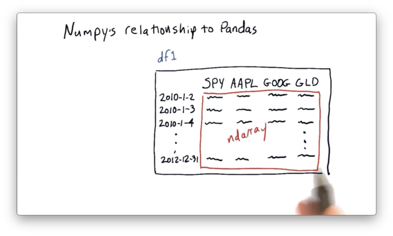
As the picture above illustrates, pandas builds df on top of an ndarray. We can retrieve the internal ndarray directly from a DataFrame df with the following code:
df.valuesWe don't have to do this explicitly, though; in fact, we can interact with df as though it were the underlying ndarray.
In other words, functionality that is available to the internal ndarray is available to df.
Of course, we create DataFrames because pandas builds a lot of great functionality on top of these ndarrays. For example, pandas provides expressive ways to access data in the array, such as symbol-based column indexing and date-based row indexing in the case of df.
Documentation
Notes on Notation
Let's look at accessing information in an ndarray nd. The basic syntax for accessing information about a row and col looks like this:
nd[row, col]NumPy uses zero-based indexing, which means that we access the very first cell using nd[0,0], not nd[1,1].
To access the cell in the fourth row and the third column, for example, we do the following:
nd[3, 2]NumPy also supports slicing. Generally, to retrieve the cells bounded by the (zero-based) index values start_row , end_row, start_col and end_col, we do the following:
nd[start_row:end_row + 1, start_col:end_col + 1]Concretely, if we want to retrieve the cells in nd that are in the first three rows and second and third columns, we do the following:
nd[0:3, 1:3]Note that NumPy slicing is upper-bound exclusive, which is why we have to add one to the end of our ranges.
If we want to select all of the rows or all of the columns in nd, we can pass in the colon by itself, like this:
nd[:, 1:3] # select all rows, second and third column
nd[0:2, :] # select first and second row, all columns
NumPy also provides syntax for negative indexing. Passing in a negative number in the slicing expression allows us to index from the "bottom" and/or "right" of nd. For example:
nd[-1, :] # select last row, all columns
nd[:, -2] # select all rows, second-to-last column
nd[-2:, :] # select second-to-last and last row, all columns
nd[:, 0:-1] # select all rows, all columns except last
Note that negative indexing is not zero-based. The last row/column is referenced by -1, not -0.
Documentation
Replace a Slice Quiz
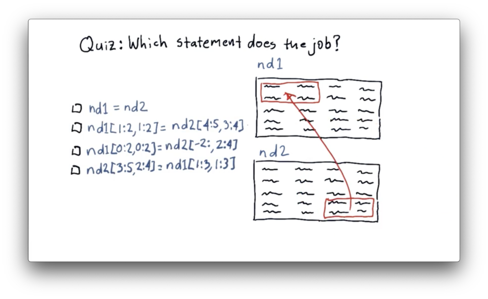
We need to move data from the last two rows and the last two columns of nd2 to the first two rows and the first two columns of nd1.
Replace a Slice Quiz Solution
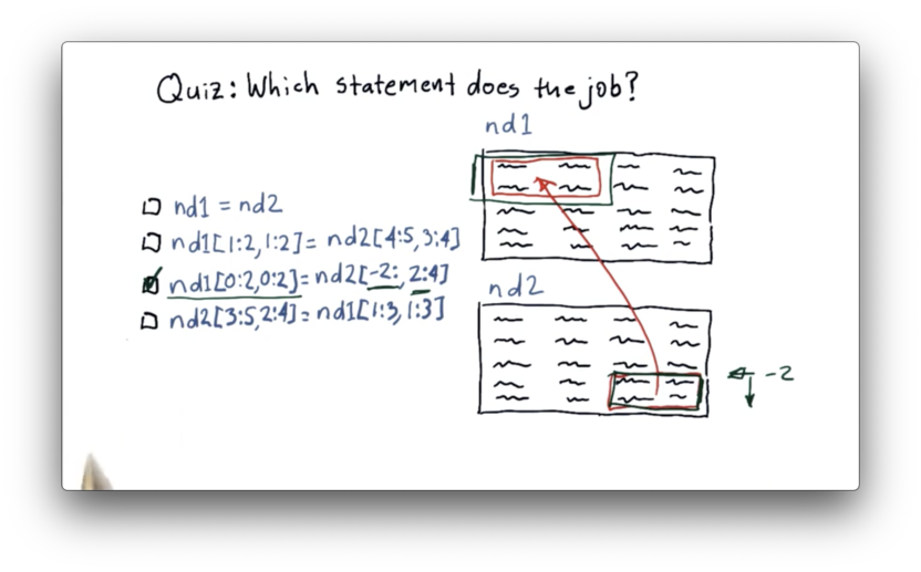
Let's first look at how we can slice nd2 to extract the data we want. We can slice the last two rows using negative indexing: -2:. We can slice the last two columns as 2:4. Remember that NumPy indexing is upper-bound exclusive.
Now let's see how we can transplant that data into nd1. We can select the first two rows of nd1 as 0:2, and we can select the first two columns as 0:2.
The complete data transfer can be accomplished with the following code:
nd1[0:2, 0:2] = nd2[-2:, 2:4]Documentation
Creating NumPy Arrays
As we said earlier, we can access the underlying NumPy array from a DataFrame through the values property. Alternatively, we can create a NumPy array from scratch:
import numpy as np
nd = np.array([2, 3, 4])
If we print nd we see the following.

We can create a two-dimensional array by passing in a list of lists:
nd = np.array([(2, 3, 4),(5, 6, 7)])If we print nd we see the following.

Documentation
Arrays with Initial Values
NumPy offers several functions for creating empty arrays with initial values. For certain computations, growing arrays incrementally can be a costly operation, so initializing empty arrays upfront may be more efficient.
We can create an empty array with shape n like so:
np.empty(n)For example, we can create an empty one-dimensional array with five elements, or an empty two-dimensional array with five rows and four columns like this:
np.empty(5)
np.empty((5, 4))
We can even create a three-dimensional array with five rows, four columns, and a depth of three:
np.empty((5, 4, 3))If we print the two-dimensional array created by np.empty((5, 4)), we see the following.
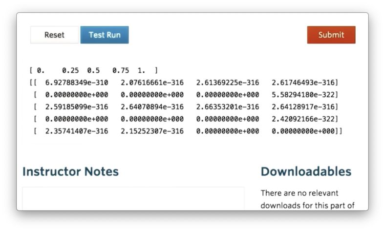
Interestingly, the empty array is not actually empty; instead, the array is filled with whatever values are present in memory at the time of array creation. Note that all of the values in the empty array are floating-point numbers.
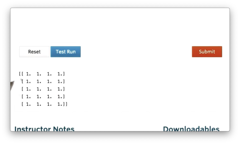
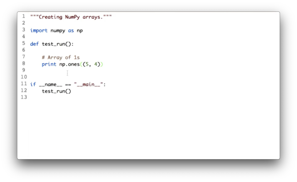
We can create an array full of ones with the np.ones function, and the following code shows how to create such an array with five rows and four columns:
np.ones((5, 4))Indeed, we see the following array when we print.
Documentation
Specify the Data Type Quiz
We saw that the elements in an array created by np.ones are floats by default. Our task here is to update the call to np.ones and pass in a parameter that tells NumPy to give us integers instead of floats.
Specify the Data Type Quiz Solution
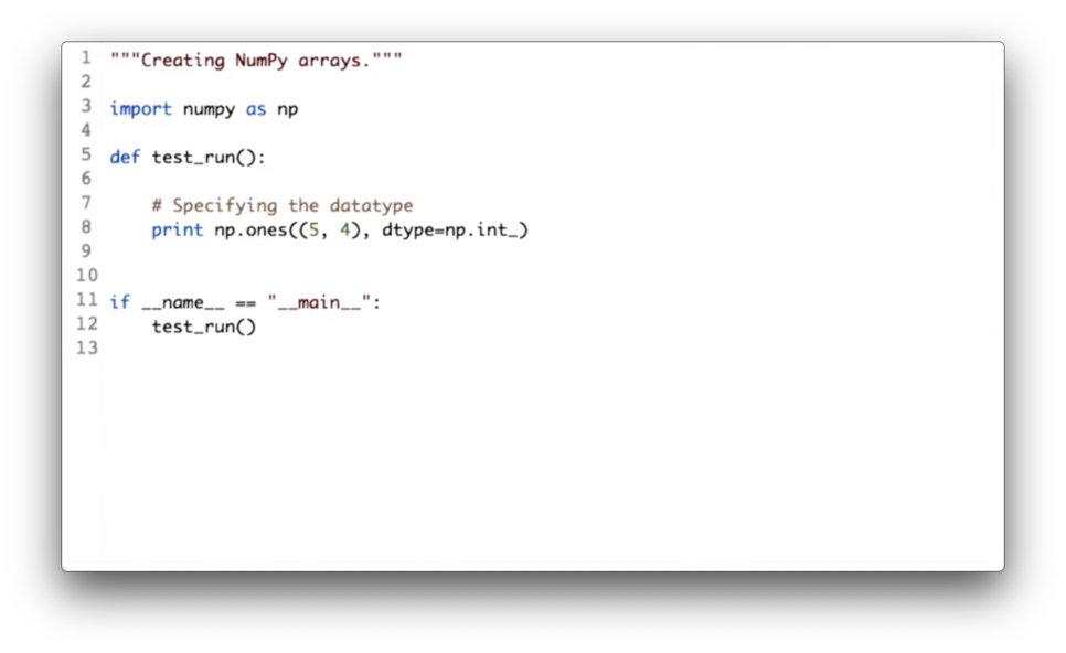
We can accomplish this change with the following code:
np.ones((5, 4), dtype=np.int_)Documentation
Generating Random Numbers
NumPy also comes with a bunch of handy functions for generating ndarrays filled with random values. These functions are defined in NumPy's random module.
The random method on the random module allows us to generate an ndarray filled with random, uniformly sampled floating-point numbers in the range of 0.0 (inclusive) to 1.0 (exclusive).
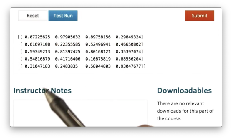
For example, we can generate such an ndarray with five rows and four columns using the following code:
np.random.random((5,4))If we print this ndarray, we see the following.
A slight variant of the random method is the rand method, which, instead of accepting a tuple corresponding to the shape, accepts a sequence of numbers describing the dimensions of the ndarray.
We can generate the same ndarray as above with rand using the following code:
np.random.rand(5, 4)NumPy exposes this syntax because it matches the more established MatLab syntax. However, we should use the random method, as the shape tuple is a consistent construct seen across NumPy.
Both rand and random sample uniformly from the range [0.0, 1.0). We can instead generate an ndarray with elements sampled from a Gaussian (normal) distribution, using the normal method.
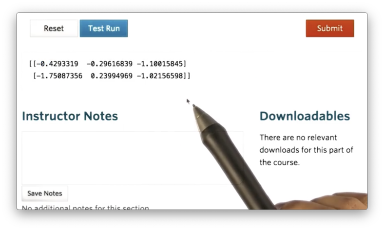
For instance, we can create such an ndarray with two rows and three columns like so:
np.random.normal(size=(2,3))If we print this ndarray, we see the following.
By default, the normal method samples from a Gaussian distribution with a mean of 0 and a standard deviation of 1. We can also sample from normal distributions parameterized by different means and standard deviations.
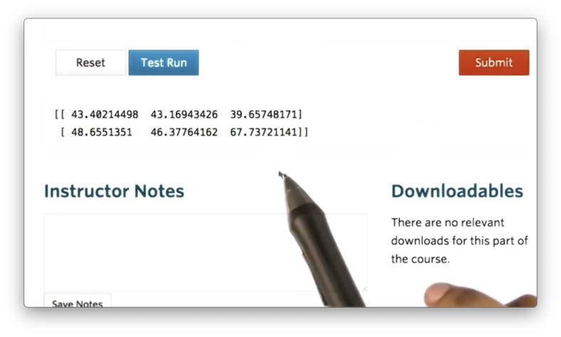
For example, we can generate an ndarray whose elements are sampled from a normal distribution with a mean of 50 and a standard deviation of 10 like this:
np.random.normal(50, 10, size=(2,3))If we print this ndarray, we see the following.
We can generate random integers using the randint method, like so:
np.random.randint(10) # single integer in [0, 10)
np.random.randint(0, 10) # single integer in [0, 10)
Additionally, we can generate an ndarray of random integers with the randint method:
# 5 random integers from [0, 10) in 1D ndarray
np.random.randint(0, 10, size=5)

# 2x3 array of random integers from [0, 10)
np.random.randint(0, 10, size=(2, 3))
If we print the previous four examples, we see the following.

Documentation
Array Attributes
Any NumPy ndarray has several attributes that describe it, in addition to the elements it contains.
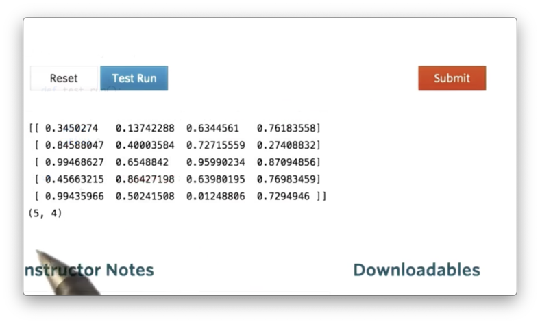
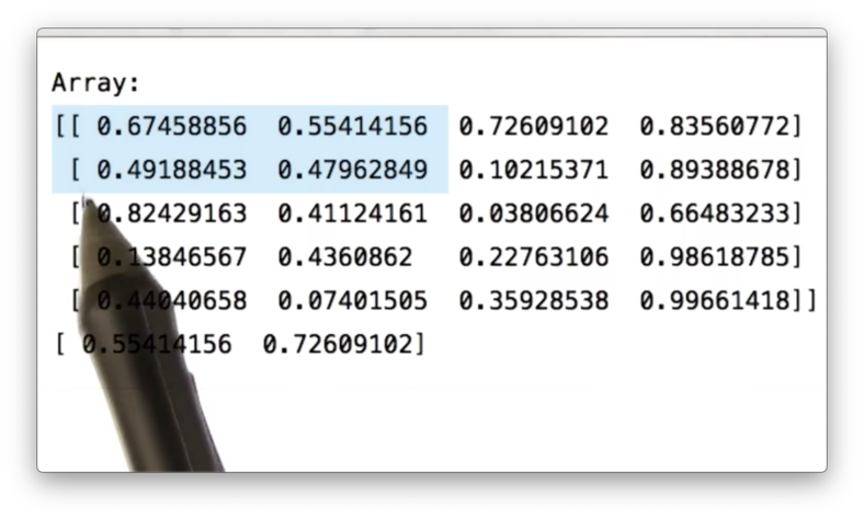
One of the most useful attributes is shape, which is essentially a tuple containing the number of rows and columns in the array. Let's create an array and access its shape:
a = np.random.random((5,4))
a.shape
If we print out a and a.shape, we see the following.
Since the shape is a Python tuple, which supports zero-based indexing, we can access just the number of rows or columns in a by indexing into the shape:
a.shape[0] # rows
a.shape[1] # columns
We can determine the number of dimensions of an ndarray nd by passing the shape tuple to the builtin len function:
len(nd.shape)We can retrieve the number of elements present in an ndarray using the size attribute. For example, we can retrieve the size of a:
a.sizeIf we print the size, we see the product of five rows and four columns.

Attributes like size and shape are useful when you need to iterate over the elements in an ndarray to perform some computation.
Finally, you can access the data type of each element using the dtype attribute of the ndarray. For example:
a.dtypeIf we print the dtype of a, we see the following.
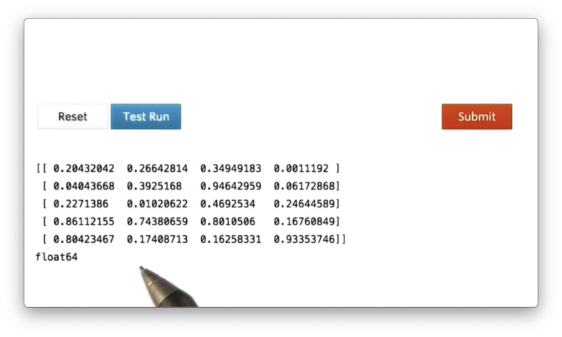
We can see that the elements of a are all 64-bit floating-point numbers.
Documentation
Operations on Ndarrays
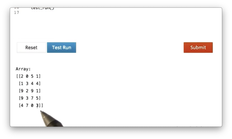
Now let's look at performing various mathematical operations on ndarrays. Let's start by creating an array a with five rows and four columns, whose elements are random integers in [0, 10):
a = np.random.randint(0, 10, size=(5,4))If we print a, we see the following.
Summing all of the elements in a is as simple as calling the sum method of a:
a.sum()If we print a with a.sum(), we see the following.

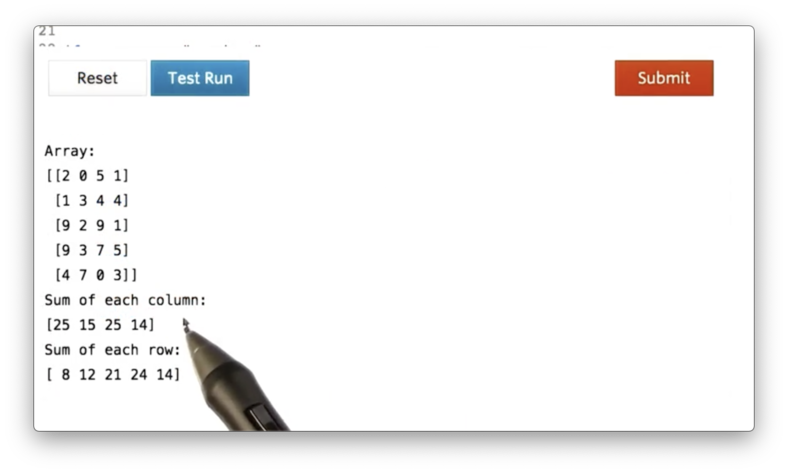
We can also calculate the sum of a in a specific direction. In other words, we can specify that we want to sum across the rows or down the columns of a.
We refer to this "direction" as an axis. The rows of an ndarray are aligned along axis zero, and the columns of an ndarray are aligned along axis one. Thus, if we want to sum all of the rows, we must sum along axis one, and if we want to sum all of the columns, we must sum down axis zero:
a.sum(axis=0) # Sum columns
a.sum(axis=1) # Sum row
If we print these sums, we see the following.
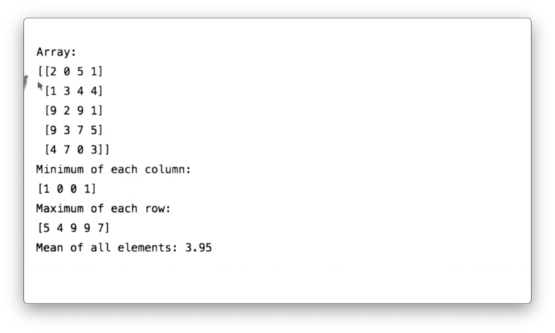
We can pull some basic statistics from an ndarray with the min, max, and mean methods, which all optionally take an axis parameter. for example:
a.min(axis=0) # column minimum
a.max(axis=1) # row maximum
a.mean() # mean of all elements
If we print out these values, we see the following.
Documentation
Locate Maximum Value Quiz
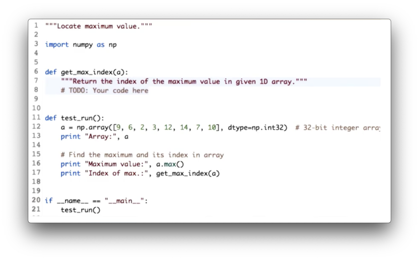
Our task is to implement the function get_max_index, which takes a one-dimensional ndarray a and returns the index of the maximum value.
Locate Maximum Value Quiz Solution
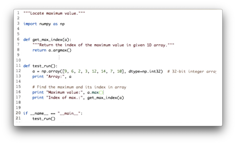
We can retrieve the index of the maximum value in a with the argmax method:
def get_max_index(a):
	return a.argmax()
Documentation
Timing Python Operations
We claimed that NumPy is very fast, and we'd like to confirm this claim. To do so, we first need to understand how to time functions in general.
We can use the time module and the time function in that library to capture the current time. We compute the time before and after executing a function and take the difference to figure out how long a function took to execute.
import time
t1 = time.time()
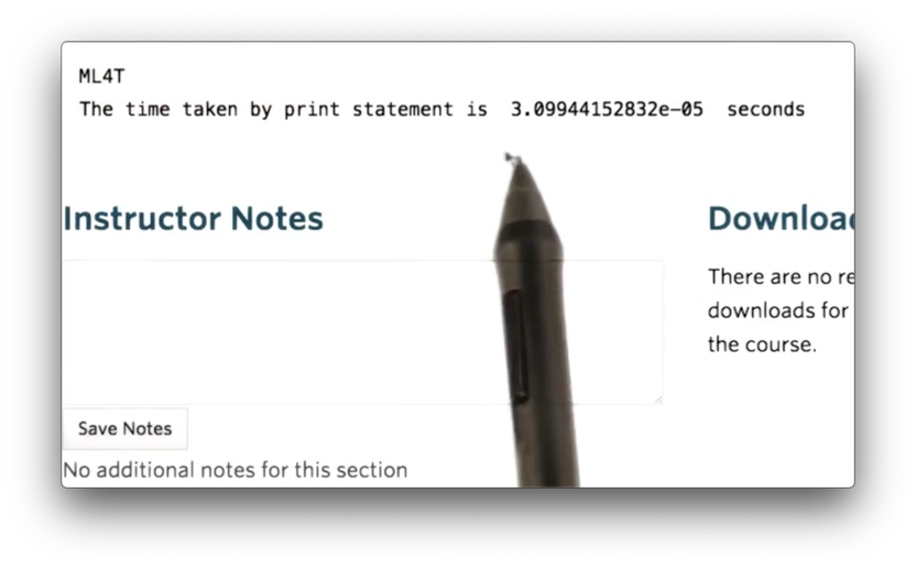
print "ML4T"
t2 = time.time()
print "The time taken by print statement is ", t2 - t1 ," seconds"If we run this code, we see the following.
Documentation
How Fast is NumPy?
Now that we know how to time an operation in Python, let's check how fast NumPy is relative to naive Python code. We start by defining a really large array, nd1:
nd1 = np.random.random((1000, 10000))We want this array to be large enough so that the differences between execution durations become unmistakably significant.
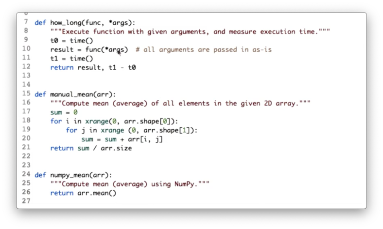
We then define the two functions that we want to test. The function numpy_mean simply calls the mean method on the passed in arr. The function manual_mean iterates over all of the elements, sums them and then divides them by the total number of elements.
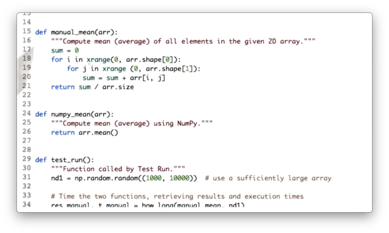
Finally, we define a how_long function, which itself receives a function func and some arguments args. The function times the execution of func(*args), and then returns the result along with the duration.
Let's check the difference in execution times.
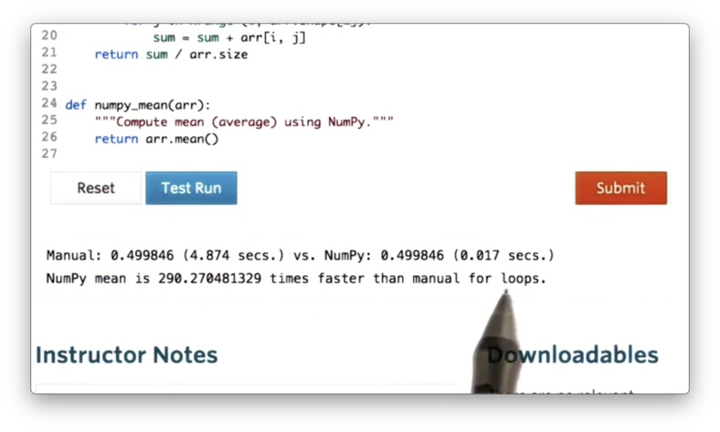
NumPy is close to 300 times faster than the simple iterative method!
Accessing Array Elements
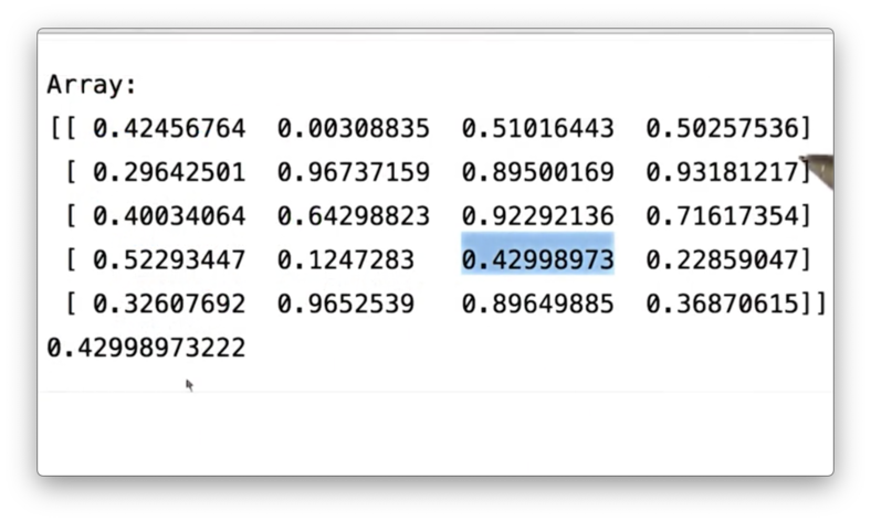
Accessing ndarray elements is straightforward. You can access a particular element by referring to its row and column number inside square brackets. For example, we can access the element in the fourth row and third column of a like so:
a[3,2]If we print out this value, we see the following.
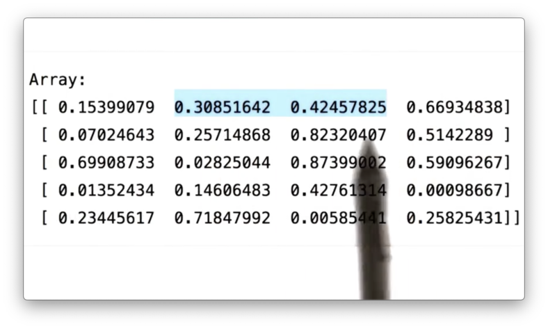
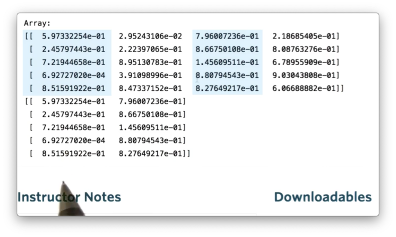
Additionally, we can access ranges of elements down columns and across rows using slicing. For instance, we can access the elements in the second and third columns of the first row of a like so:
a[0, 1:3]If we print this slice, we see the following.
We can combine row and column slicing to select, for example, the elements in the first two rows and first two columns of a like so:
a[0:2, 0:2]If we print this slice, we see the following.
So far, we have only seen slice syntax like x:y, which defines a slice starting at row/column x and ending at row/column y - 1. We can specify a third parameter, z, which defines the step size.
For example, we can select all rows, but only the first and third columns of a like this:
a[:, 0:3:2]If we print this slice, we see the following.
Documentation
Modifying Array Elements
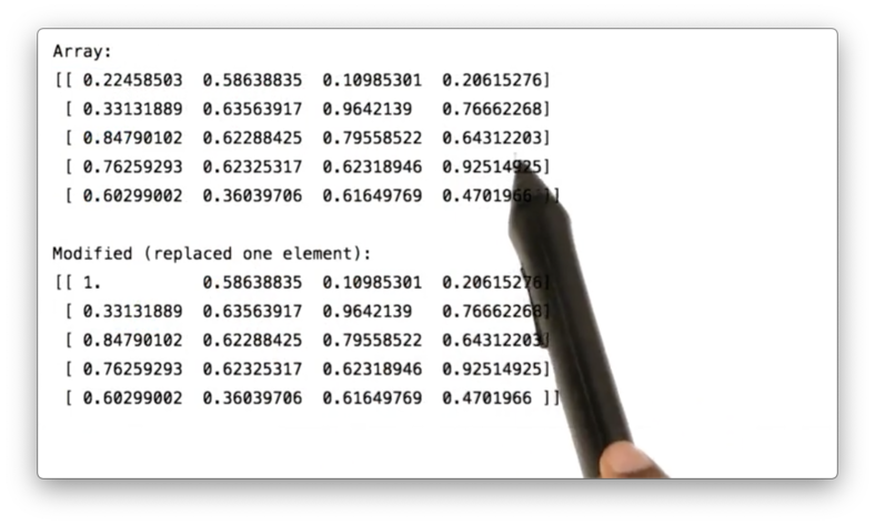
As well as accessing elements in ndarrays, we can also assign values to specific locations in ndarrays. As a simple example, we can set the first element in a to 1 like this:
a[0, 0] = 1Let's look at a before and after the assignment.
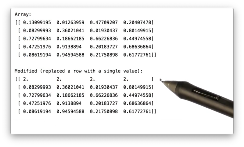
We can use slicing for assignment as well as access. For example, we can set all of the elements in the first row of a like this:
a[0, :] = 2If we print a, we see the following.
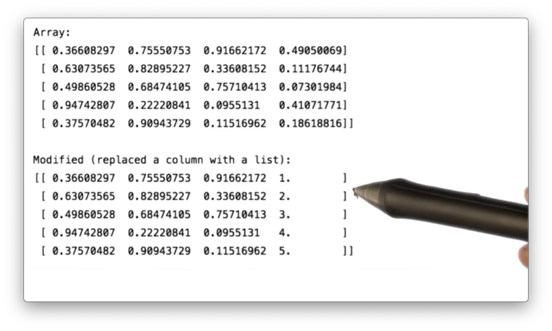
We don't have to set all of the elements in a row or column to the same value. If we assign a column or row to a list, each element will be set to the corresponding value in the list.
For example, we can set the fourth column of a to the values 1 through 5 with the following assignment:
a[:, 3] = [1, 2, 3, 4, 5]If we print a, we see the following.
Documentation
Indexing an Array with Another Array
An ndarray can also be indexed with another ndarray. To demonstrate this, let's first create an ndarray a:
a = np.random.rand(5)Next, let's create an ndarray indices whose elements represent the indices of the values we want to retrieve from a:
indices = np.array([1, 1, 2, 3])We can retrieve the values in a at the indices in indices like so:
a[indices]This expression is saying the following: for each element in indices retrieve the element in a at that index.
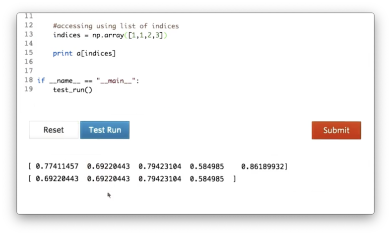
Indeed, we can see that our resulting array contains the elements of a at indices 1, 1, 2, and 3.
Documentation
Boolean or "Mask" Index Arrays
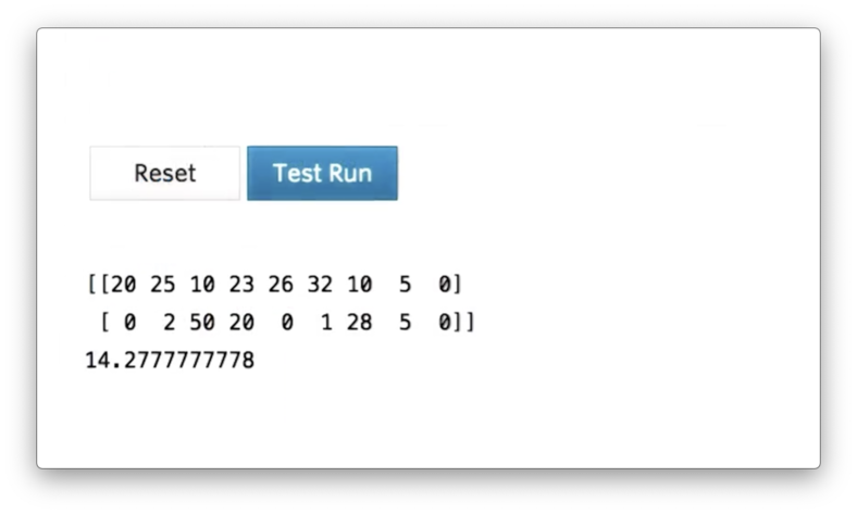
Let's see how we can retrieve all of the values from an ndarray that are less than the mean of that array. First, we construct our two-dimensional ndarray a and calculate the mean:
a = np.array([
(20, 25, 10, 23, 26, 32, 10, 5, 0)
(0, 2, 50, 20, 0, 1, 28, 5, 0)
])
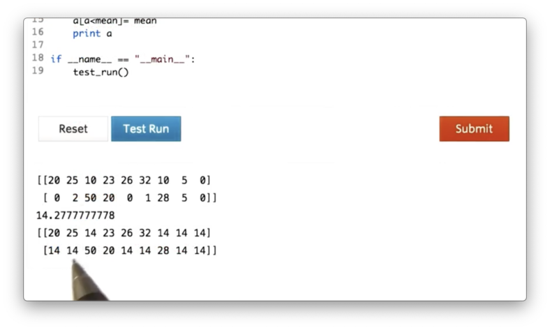
mean = a.mean()If we print a and mean, we see the following.
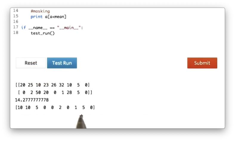
While we can technically run a for loop over the elements in a and keep only those values less than 14.2, there is a cleaner way:
a[a < mean]We can interpret this expression as: for each value a_i in a, compare a_i with mean and retain the value if a_i > mean.
If we print the output of the expression, we see the following ndarray.
Additionally, we can use this masking technique to set the values of a that are less than mean to mean:
a[a < mean] = meanIf we print a now, we see the following.
Documentation
Arithmetic Operations
Arithmetic operations on ndarrays are always applied element-wise. Let's first create an ndarray a:
a = np.array([
(1, 2, 3, 4, 5),
(10, 20, 30, 40, 50)
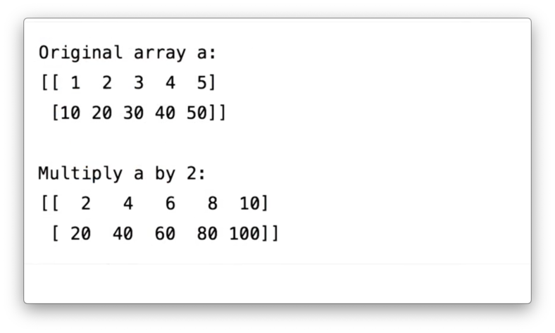
])We can multiply each element in a by two:
2 * aIf we print the result of this multiplication, we see the following.
We can divide each element in a by two:
a / 2If we print the result of this division, we see the following.
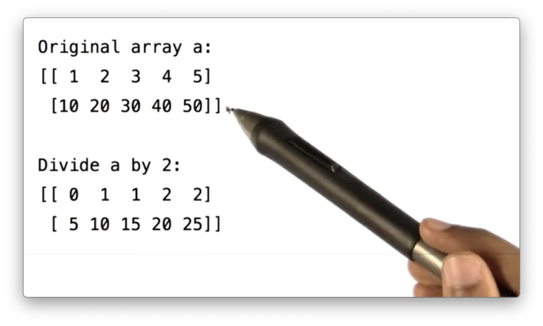
Note that both the divisor and the elements in the ndarray are integers. As a result, integer division (rounding down, roughly) is performed, which is why 1 / 2 equals 0.
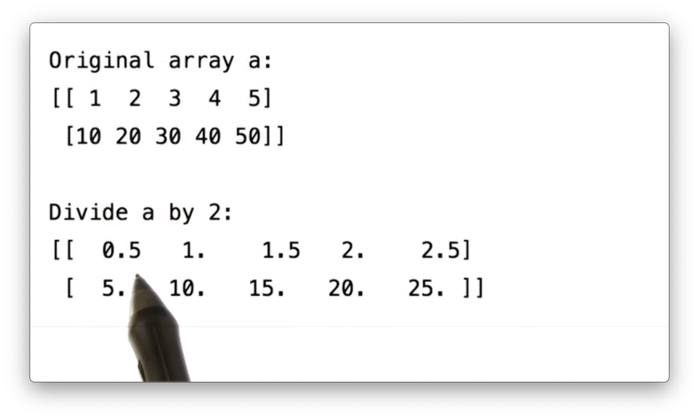
We can cast the resulting array into float values by ensuring that the divisor is a float:
a / 2.0If we print the result of this division, we see the following.
Our arithmetic capabilities are not limited to just operations between ndarrays and scalar values. We can also perform operations that combine two ndarrays. Let's create a second ndarray b.
a = np.array([
    (100, 200, 300, 400, 500),
    (1, 2, 3, 4, 5)
])
We can add a and b:
a + bIf we print the result of this addition, we see the following.
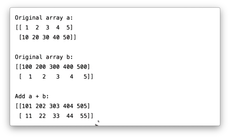
Note that the shape of a and b should be similar before trying to perform operations that involve both ndarrays; otherwise, NumPy will throw an error.
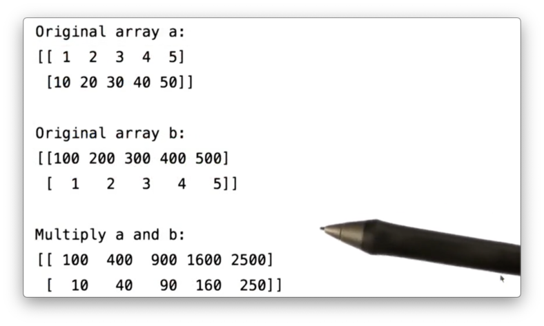
The multiplication operator allows us to multiply two ndarrays in an element-wise manner. Note that other languages commonly use the multiplication operator to signify the dot product. NumPy does not do this.
We can multiply a and b in an element-wise fashion:
a * bIf we print the result of this multiplication, we see the following.
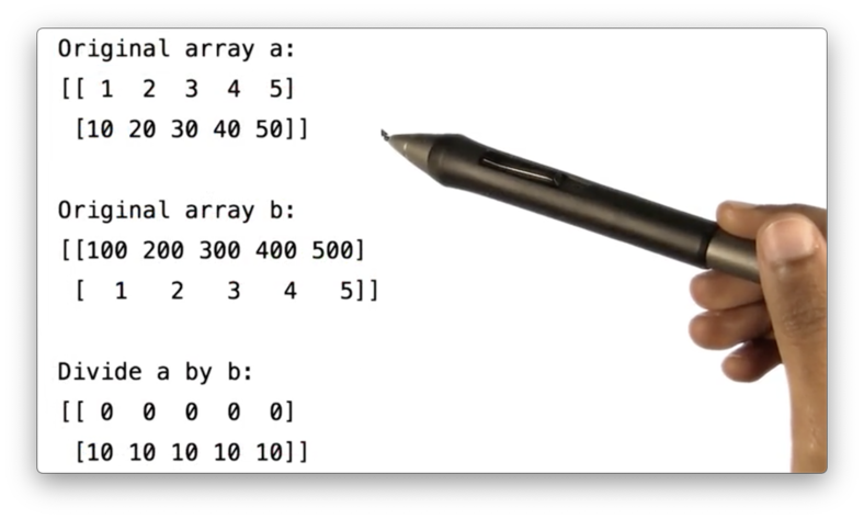
We can divide a by b:
a / b If we print the result of this division, we see the following. Remember that we are doing integer division here.
OMSCS Notes is made with in NYC by Matt Schlenker.
Copyright © 2019-2023. All rights reserved.
privacy policy