Operating Systems
Scheduling
28 minute read
Notice a tyop typo? Please submit an issue or open a PR.
Scheduling
Scheduling Overview
The CPU scheduler decides how and when the processes (and their threads) access the shared CPUs. The scheduler concerns the scheduling of both user level tasks and kernel level tasks.
The scheduler selects one of the tasks in the ready queue and then schedules it on the CPU. Tasks may become ready a number of different ways.
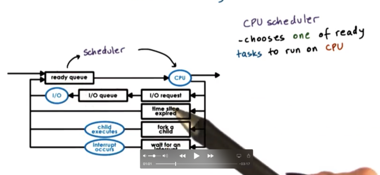
Whenever the CPU becomes idle, we need to run the scheduler. For example, if a task makes an I/O request and is placed on the wait queue for that device, the scheduler has to select a new task from the ready queue to run on the CPU.
A common way that schedulers share time within the system is by giving each task some amount of time on the CPU. This is known as a timeslice. When a timeslice expires, the scheduler must be run.
Once the scheduler selects a task to be scheduled, that task is dispatched onto the CPU. The operating system context switches to the new task, enters user mode, sets the program counter, and execution begins.
In summary, the objective of the OS scheduler is to choose the next task to run from the ready queue.
How do we decide which task to be selected? This depends on the scheduling policy/algorithm. How does the scheduler accomplish its job? This depends very much on the structure of ready queue, also known as a runqueue. The decision of the runqueue and the scheduling algorithm are tightly coupled: a data structure that is optimized for one algorithm may be a poor choice for implementing another.
Run To Completion Scheduling
Run To Completion scheduling assumes that once a task is assigned to a CPU, it will run on that CPU until it is finished.
For the purposes of discussion, it's necessary to make some assumptions. First, we can assume that we have a group of tasks that need to be scheduled. Second, we can assume that we know the execution times of the tasks. Third, we can assume that there is no preemption in the system. Fourth, assume that there is a single CPU.
When it comes to comparing schedulers, some common metrics include:
- throughput
- average job completion time
- average job wait time
- CPU utilization
The first and the simplest algorithm is First Come First Serve (FCFS). In this algorithm, the tasks are simply scheduled in the order in which they arrive. When a task completes, the scheduler will pick the next task in order.
A simple way to organize these tasks would be a queue structure, in which the tasks can be enqueued to the back of the queue, and dequeued from the front of the queue by the scheduler in a FIFO manner. All the scheduler needs to know is the head of the queue, and how to dequeue tasks.
Let's look at a scenario with three threads: T1, T2, T3. T1 has a task that takes 1 second, T2 has a task that takes 10 seconds, and T3 has a task that takes 1 second. Let's assume that T1 arrives before T2, which arrives before T3.
For this example, the throughput is 3 tasks over 12 seconds, or 0.25 tasks per second. The average completion time is (1 second + 11 seconds + 12 seconds) / 3, or 8 seconds. The average wait time is (0 seconds + 1 second + 11 seconds) / 3, or 4 seconds.
We can improve our metrics by changing our algorithm. Instead of FCFS we can try shortest job first (SJF), which schedules jobs in order of their execution time.
With this algorithm, it doesn't really make sense for the runqueue to be a FIFO queue any more. We need to find the shortest task in the queue, so we may need to change our queue to be an ordered queue. This makes the enqueue step more laborious. Alternatively, we can use a tree structure to maintain the runqueue. Depending on how we rebalance the tree every time we add a new task, we can easily find the node containing the shortest job. The runqueue doesn't have to be queue!
Preemptive Scheduling: SJF + Preempt
Let's remove the assumption that a task cannot be interrupted once its execution has started. Let's also relax the assumption that tasks must all arrive at the same time.
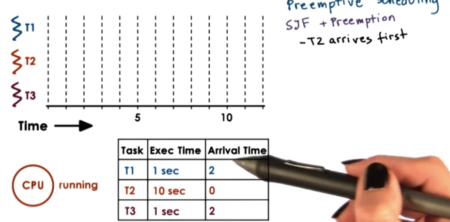
When T2 arrives, it is the only task in the system, so the scheduler will schedule it. When T1 and T3 arrive, T2 should be preempted, in line with our SJF policy. The execution of the rest of the scenario is as follows.
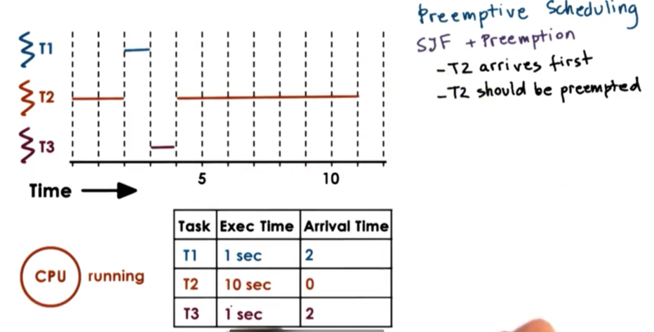
Whenever tasks enter the runqueue, the scheduler needs to be invoked so that it can invoke the new task's runtime, and make a decision as to whether it should preempt the currently executing task.
We are still holding our assumption that we know the execution time of the task. In reality, this is not really a fair assumption, as the execution time depends on many different things that may be out of our perception. We can generate heuristics about running time based on execution times that have been recorded for similar jobs in the past. We can think about how long a task took to run the very last time or the average execution time over the past n times (a windowed average).
Preemptive Scheduling: Priority
Instead of looking at execution time when making scheduling decisions, as we do in SJF, we can look at task priority levels. It is common for different tasks to have different priorities. For example, it is common that kernel level tasks that manage critical system components will have higher priority than tasks that support user applications.
When scheduling based on priority, the scheduler must run the highest priority task next. As a precondition of this policy, the scheduler must be able to preempt lower priority tasks when a high priority task enters the runqueue.
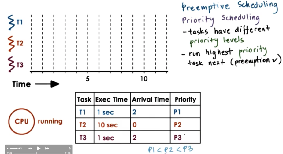
We start with the execution of T2, as it is the only thread in the system. Once T3 and T1 are ready, T2 is preempted. T3 is scheduled as it has the highest priority, and it runs to completion. T2 is scheduled again - as it has higher priority than T1 - and runs to completion. Finally, T1 is scheduled and runs to completion.
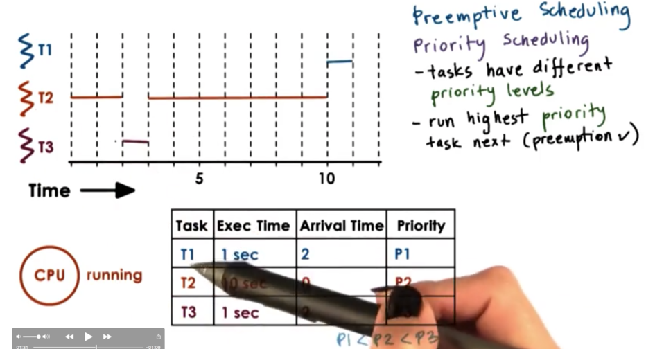
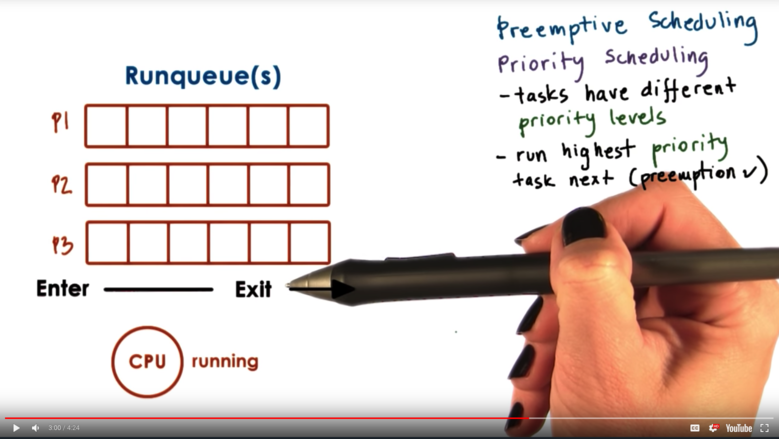
Our scheduler now not only needs to know which tasks are runnable, but also each task's priority. An effective way to be able to quickly tell a task's priority is to maintain a separate runqueue for each priority level. As a result, the scheduler can just empty queues by priority level.
One dangerous situation that can occur with priority scheduling is starvation, in which a low priority tasks is essentially never scheduled because higher priority tasks continually enter the system and take precedence.
One mechanism to protect against starvation is priority aging. In priority aging, the priority of a task is not just the numerical priority, but rather a function of the actual priority and the amount of time the task has spent in the runqueue. This way, older tasks are effectively promoted to higher priority to ensure that they are scheduled in a reasonable amount of time.
Priority Inversion
Consider the following setup assuming an SJF policy with priority, where P3 < P2 < P1.
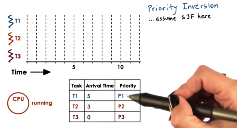
Initially, T3 is the only task in the system, so it begins executing. Suppose it acquires a mutex. T2 now arrives, which has higher priority than T3, so T3 is preempted and T2 begins to execute. Now T1 arrives and preempts T2. Suppose T1 needs the lock that T3 holds. T1 gets put on the wait queue for the lock and T2 executes. T2 finishes and T3 executes. Once T3 finishes and unlocks the mutex, T1 can finally run.
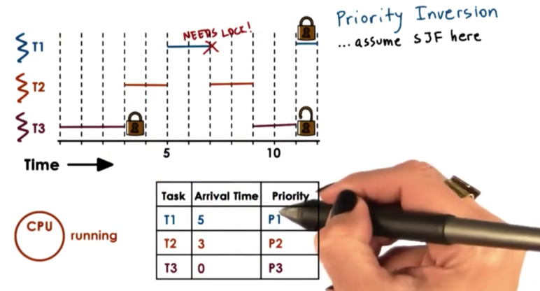
We see that we have a case of priority inversion here because T1 which has the highest priority is now waiting on T3 which has the lowest priority. The order of execution should have been T1, T2, T3, but instead was T2, T3, T1.
A solution to this problem would have been to temporarily boost the priority of the mutex owner. When T1 needs to acquire the lock owned by the T3, T3 should have its priority boosted to P1, so it would be scheduled on the CPU. Once T3 releases its mutex, T3 should have its priority dropped back to P3, so T1 can now execute, as T1 is the task with the actual highest priority.
We can now see why it is important to keep track of the current owner of the mutex in the mutex data structure.
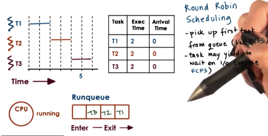
Round Robin Scheduling
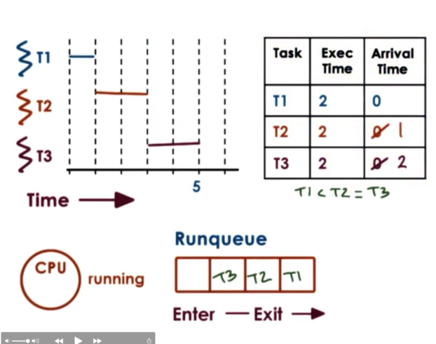
When it comes to running jobs with the same priority there are alternatives to FCFS and SJF. A popular option is round robin scheduling. Consider the following scenario.
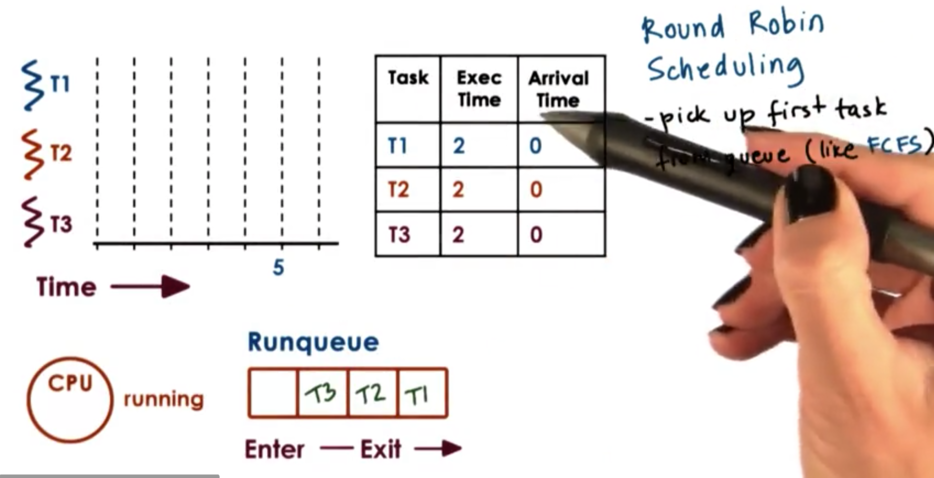
We have three tasks that all arrive at the same time and are all present in the runqueue. We first remove T1 from the queue and schedule it on the CPU. When T1 completes, T2 will be removed from the queue and scheduled on the CPU. When T2 completes, T3 will be removed from the queue and scheduled on the CPU.
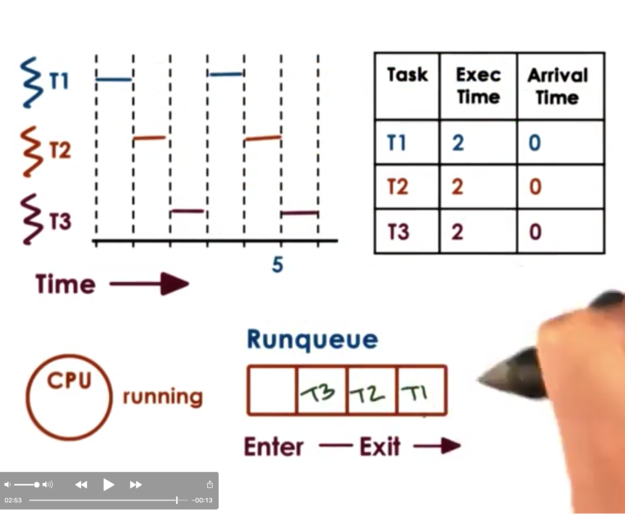
We can generalize round robin to include priorities as well.
A further modification that makes sense with round robin is not to wait until the tasks explicitly yield, but instead to interrupt them in order to mix in all the tasks in the system at the same time. For example, we would give each task a window of one time unit before interrupting it to schedule a new task. We call this mechanism timeslicing.
Timesharing and Timeslices
A timeslice (also known as a time quantum) is the maximum amount of uninterrupted time that can be given to a task. A task may run for a smaller amount of time than what the timeslice specifies. If the task needs to wait on an I/O operation, or synchronize with another task, the task will execute for less than its timeslice before it is placed on the appropriate queue and preempted. Also, if a higher priority tasks becomes runnable before a lower priority task's timeslice has expired, the lower priority task will be preempted.
The use of timeslices allows for the tasks to be interleaved. That is, they will be timesharing the CPU. For I/O bound tasks, this is not super critical, as these tasks will often be placed on wait queues. However, for CPU bound tasks, timeslices are the only way that we can achieve timesharing.
Let's compare round robin scheduling with a timeslice of 1 to the FCFS and SJF algorithms across the metrics of throughput, average wait, and average completion.
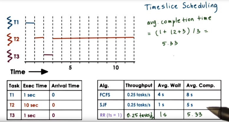
T1 executes for one second, and is completed. T2 executes for one second and is preempted by T3. T3 executes for 1 second and is completed. T2 now executes for 9 seconds (no other tasks are present to preempt it), and it completes.
For metrics, our throughput stays the same, and our average wait and average completion time are on par with SJF, but without needing the a priori knowledge of execution times, which was said was unfeasible in a real system.
Some of the benefits of timeslicing are that the short tasks finish sooner, the scheduler is more responsive to changes in the system, and that lengthy I/O operations can be initiated sooner.
The downside of timeslicing is the overhead. We have exaggerated in our graphs that there is no latency between tasks, but this is not the case. Timeslicing takes time: we have to interrupt the running task, we have to execute the scheduler, and we have to context switch to the new task.
Even when there are no other runnable tasks in the system, as with the case of T2 above after T=3, the scheduler will still be run at timeslice intervals. That being said, there will be no context switching so the overhead will not be as great when the current task does not need to be preempted.
If we consider the overheads when we compute our metrics, we can see that our total time will increase slightly, so our throughput will go down. As well, each task will have to wait just a little longer to start, so our wait time and our completion time will increase.
As long as the timeslice is significantly longer than the amount of time it takes to context switch, we should be able to minimize the overheads of context switching.
How Long Should a Timeslice Be
Timeslices provide benefits to the system, but also come with certain overheads. The balance of the benefits and the overheads will inform the length of the timeslice. The answer is different for I/O bound tasks vs. CPU bound tasks.
CPU Bound Timeslice Length
Let's consider two CPU bound tasks that each take 10 seconds to complete. Let's assume that the time to context switch is 0.1 seconds. Let's consider a timeslice value of 1 second and a timeslice value of 5 seconds.
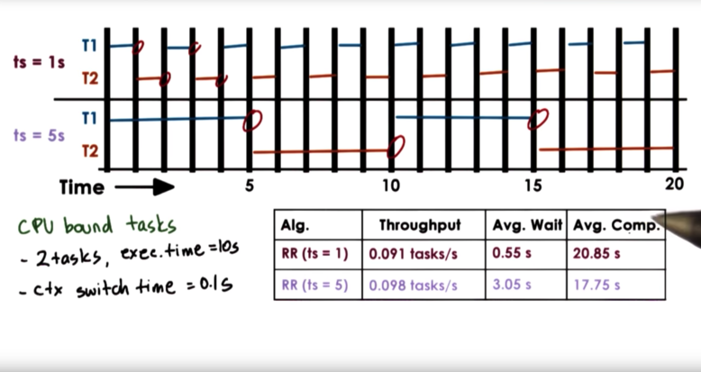
With a smaller timeslice value, we have to pay the time cost of context switching more frequently. This will degrade our throughput and our average completion time. That being said, smaller timeslices mean that tasks are started sooner, so our average wait time is better when we have smaller timeslices.
The user cannot really perceive when a CPU bound task starts, so average wait time is not super important for CPU bound tasks. The user cares when a CPU bound task completes.
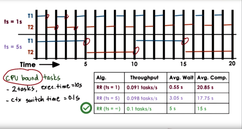
For CPU bound tasks, we are better off choosing a larger timeslice. In fact, if our timeslice value was infinite - that is to say we never preempt tasks - our metrics would be best.
I/O Bound Timeslice Length
Let's consider two I/O bound tasks that each take 10 seconds to complete. Let's assume that the time to context switch is 0.1 seconds. Let's assume that each task issues an I/O request every 1 second, and that I/O completes in every 0.5 seconds. Let's consider a timeslice value of 1 second and a timeslice value of 5 seconds.
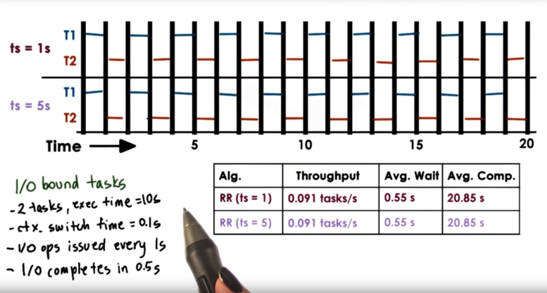
In both cases, regardless of the timeslice, each task is yielding the CPU after every second of operation - when it makes its I/O request. There isn't really any preemption going on. Thus the execution graphs and the metrics for timeslice values of 1 second and 5 seconds are identical.
Let's change the scenario and assume only T2 is I/O bound. T1 is now CPU bound.
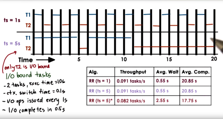
The metrics for a timeslice value of 1 second do not change. The only function difference we have is that T1 is now explicitly preempted when its timeslice expires as opposed to before when T1 yielded the CPU after issuing its I/O request.
The metrics for a timeslice value of 5 seconds do change. T1 runs until its timeslice expires at T=5. T2 then runs for only 1 second until it issues its I/O request. T1 then runs again for 5 seconds and completes. Finally T1 runs and completes.
Note that the I/O latency of T2 can no longer be hidden, which means that the total execution time of these operations is extended (graph is wrong), which means that the throughput suffers. The average wait time suffers as well, because T2 now has to wait 5 seconds for T1's timeslice to expire. Finally, average completion time is improved, as T1 can completely exhaust its timeslice and finish quickly.
For I/O bound tasks, we want a smaller timeslice. We can keep throughput up and average wait time down with a smaller timeslice. As well, we can maximize device utilization with a smaller timeslice, as we can quickly switch between different tasks issuing I/O requests.
Summarizing Timeslice Length
CPU bound tasks prefer longer timeslices as this limits the number of context switching overheads that the scheduling will introduce. This ensures that CPU utilization and throughput will be as high as possible.
On the other hand, I/O bound tasks prefer short timeslices. This allows I/O bound tasks to issue I/O requests as soon as possible, and as a result this keeps CPU and device utilization high and well improves user-perceived performance (remember wait times are low).
Runqueue Data Structure
The runqueue data structure is only logically a queue. It can be implemented as multiple queues or even a tree. What's important is that the data structure is designed so that the scheduler can easily determine which task should be scheduled next.
For example, if we want I/O and CPU bound tasks to have different timeslice values, we can either place I/O and CPU bound tasks in the same runqueue and have the scheduler check the type, or we can place them in separate runqueues.
One common data structure is a multi queue structure that maintains multiple distinct queues, each differentiated by their timeslice value. I/O intensive tasks will be associated with the queue with the smallest timeslice values, while CPU intensive tasks will be associated with the queue with the largest timeslice values.
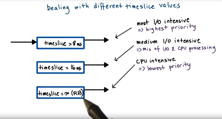
This solution is beneficial because it provides timeslicing benefits for I/O bound tasks, while also avoid timeslicing overheads for CPU bound tasks.
How do you know if a task is CPU or I/O intensive?
We can use history based heuristics to determine what a task has done in the past as a way to inform what it might do in the future. However, this doesn't help us make decisions about new tasks or tasks that have dynamic behaviors.
To help make these decisions, we will need to move tasks between queues.
When a new task enters the system, we will place it on the topmost queue (the one with the lowest timeslice). If the task yields before the timeslice has expired, we have made a good choice! We will place this task back on this queue when it becomes runnable again. If the task has to be preempted, this implies that the task was more CPU intensive than we thought, and we push it down to a queue with a longer timeslice. If the task has to be preempted still, we can push the task down even further, to the bottom queue.
If a task in a lower queue begins to frequently release the CPU due to I/O waits, the scheduler may boost the priority of that task and place it in a queue with a smaller timeslice.
The resulting data structure is called the multi-level feedback queue.
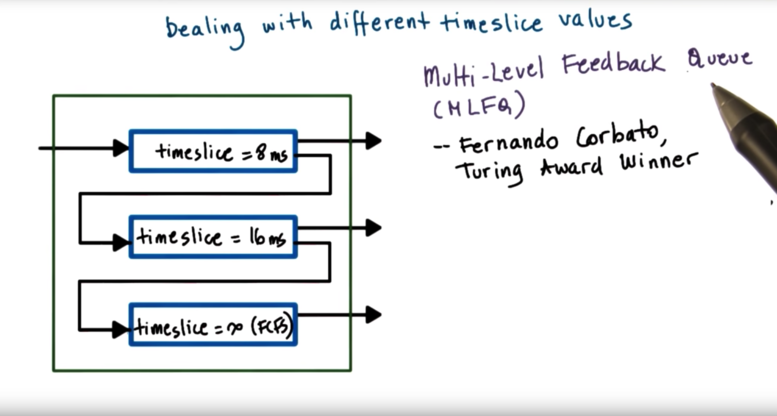
The MLFQ is not just a group of priority queues. There are different scheduling policies associated with each level. Importantly, this data structure provides feedback on a task, and helps the scheduler understand over time which queue a task belongs to given the makeup of tasks in the system.
Linux O(1) Scheduler
The Linux O(1) scheduler gets its name from the fact that it can add/select a task in constant time, regardless of the number of tasks in the system. It is a preemptive, priority-based scheduler, with 140 priority levels. The priority levels are broken into two classes: priorities from 0 to 99 are for real-time tasks, while 100 - 139 are for timesharing tasks.
User processes have priorities in the timesharing class, with the default priority in the middle at 120. Priority levels can be adjusted with so-called nice values which span from -20 to 19, corresponding to 120 - 20 to 120 + 19. There is a system call to adjust the priority of a user process.
The O(1) scheduler borrows from the MLFQ scheduler in that each priority level is associated with a different timeslice value. As well, the O(1) scheduler uses feedback from how tasks behaved in the past in order to understand how to prioritize tasks in the future.
The scheduler assigns the smallest timeslice values to the low-priority, CPU bound tasks, and assigns the largest timeslice values to the more interactive tasks.
The feedback for the task depends on how long the task spent sleeping during its timeslice. Sleeping refers to time spent idling or waiting. If a task spends more time sleeping, this means it is a more interactive tasks, and its priority is boosted (priority - 5). If a task spends less time sleeping, this means it is a more computationally intensive task, and its priority is lowered (priority + 5).
The runqueue in the O(1) scheduler is implemented as two arrays of tasks. Each array elements points to the first runnable task at that priority level.
The two arrays are active and expired.
The active list is the primary one that the scheduler uses to select the next task to run. It takes constant time to add a task, as it takes constant time to index into the array and then follow the pointer to the end of the task list to enqueue the task. It takes constant time to select a task because the scheduler relies on certain instructions that return the first set bit in a sequence of bits. If the sequence of bits corresponds to the priority levels, and a set bit means that there are tasks at that level, then it will take a constant amount of time to run those instructions to detect what is the priority level that has certain tasks on it. Once that position is known, it takes a constant amount of time to index into the array and select the first task from the task list.
If a task yields the CPU to wait on an event or is preempted due to a higher priority task becoming runnable, the time it has spent on the CPU is compared to the timeslice. If it is less than the timeslice, the task is placed back on the active queue for that priority level.
Only after the entire timeslice has been exhausted will the task move to the expired array. The expired array contains the inactive tasks. This means that the scheduler will not schedule tasks from this array while there are still tasks in the active array. Once there are no more tasks in the active array, the empty and the active array will be swapped.
This sheds a little bit of light as to why the lowest priority tasks have the smallest timeslices. Remember, we had originally thought to give the lowest priority, CPU intensive tasks the largest timeslices. In this case, however, giving the lowest priority tasks the smallest timeslices ensures that low priority tasks - which only run after all higher priority tasks expire - do not block the higher priority tasks for too long. The lower priority tasks get their small window to accomplish their work, and then quickly yield back to more important tasks.
The O(1) scheduler was introduced in Linux 2.5. Despite its constant time add/select functionality, though, this scheduler was not performant enough to keep up with the realtime needs of new applications, like Skype, for instance. For this reason, the O(1) scheduler was replaced by the completely fair scheduler (CFS) in Linux 2.6.23, which is now the default scheduler.
Linux CFS Scheduler
One problem with the O(1) is that once a task enters the expired queue, it will not get a chance to run again until all other tasks in the active queue have executed for their timeslices. This is a problem for interactive tasks, introducing jitter into interactions that should appear seamless.
In addition, the scheduler in general doesn't make any fairness guarantees. Intuitively, fairness is the concept that in a given time interval, a task should be able to run for an amount of time that is relative to its priority.
As a replacement for the O(1) scheduler, the CFS scheduler was introduced. CFS is now the default scheduler for non-realtime tasks in Linux.
CFS uses a red-black tree as a runqueue structure. Red black trees are self-balancing trees, which ensure that all of the paths from the root of the tree to the leaves are approximately the same size.
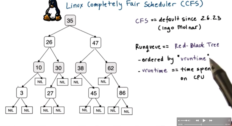
Tasks are ordered in the tree based on the amount of time that they spent running on the CPU, a quantity known as vruntime (virtual runtime). CFS tracks this quantity to the nanosecond.
This runqueue has the property that for a given node, all nodes to the left have lower vruntimes and therefore need to be scheduled sooner, while all nodes to the right, have larger vruntimes and therefore can wait longer.
The CFS algorithm always schedules the node with the least amount of vruntime in the system, which is typically the leftmost node of the tree. Periodically, CFS will increment the vruntime of the task that is currently executing on the CPU, at which point it will compare this vruntime with the vruntime of the leftmost task in the tree. If the currently running task has a smaller vruntime than the leftmost node, it will keep running; otherwise, it will be preempted in favor of the leftmost node, and will be inserted appropriately back into the tree.
For lower priority tasks the vruntime will be updated more frequently; that is, the scheduler will often check if it is time to preempt a lower priority task. We can think of time moving more quickly for lower priority tasks. For higher priority tasks the vruntime will be updated less frequently; that is, the scheduler will rarely check if it is time to preempt a higher priority task. We can think of time moving more slowly for higher priority tasks.
In summary, task selection from the runqueue takes constant time. Adding a task to the runqueue takes log time relative to the total number of tasks in the system.
It is possible that the log(n) performance of the addition step may limit the use of this scheduler as the number of tasks a system can handler increases past a certain threshold. At some point, the search may be on for a fair scheduler than can select and add in constant time.
Scheduling on Multiprocessors
Before we can talk about scheduling on multiprocessor systems, it is important to understand the architecture of multiprocessor systems.
In a shared memory multiprocessor, there are multiple CPUs. Each CPU has its own private L1/L2 cache, as well as a last-level cache (LLC) which may or may not be shared amongst the CPUs. Finally, there is system memory (DRAM) which is shared across the CPUs.
In a multicore system, each CPU can have multiple internal cores. Each core has it's own private L1/L2 cache, and the CPU as a whole shares an LLC. DRAM is present in this system as well.
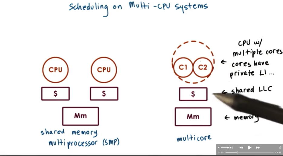
As far as the operating system is concerned, it sees all of the CPUs and all of the cores in the CPUs as entities onto which it can schedule tasks.
Since the performance of processes/threads is highly dependent on the amount of execution state that is present in the CPU cache - as opposed to main memory - it makes sense that we would want to schedule tasks on to CPUs such that we can maximize how "hot" we can keep our CPU caches. To achieve this, we want to schedule our tasks back on the same CPUs they had been executing on in the past. This is known as cache affinity.
To achieve cache affinity, we can have a hierarchical scheduling architecture which maintains a load balancing component that is responsible for dividing the tasks among CPUs. Each CPU then has its own scheduler with its own runqueue, and is responsible for scheduling tasks on that CPU exclusively.
To load balance across the CPUs, we can look at the length of each of the runqueues to ensure one is not too much longer than the other. In addition, we can detect when a CPU is idle, and rebalance some of the work from the other queues on to the queue associated with the idle CPU.
In addition to having multiple processors, it is possible to have multiple memory nodes. The CPUs and the memory nodes will be connected via some physical interconnect. In most configurations it is common that a memory node will be closer to a socket of multiple processors, which means that access to this memory node from those processors is faster than accessing some remote memory node. We call these platforms non-uniform memory access (NUMA) platforms.
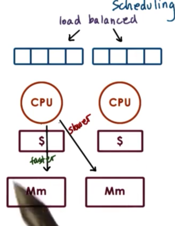
From a scheduling perspective, what makes sense is to keep tasks on the CPU closest to the memory node where their state is, in order to maximize the speed of memory access. We refer to this as NUMA-aware scheduling.
Hyperthreading
The reason why we have to context switch among threads is because the CPU only has one set of registers to describe an execution context. Over time, hardware architects have realized they can hide some of the latency associated with context switching. One of the ways that this has been achieved is to have CPUs with multiple sets of registers where each set of registers can describe the context of a separate thread.
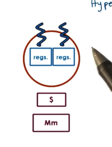
We call this hyperthreading. In hyperthreading, we have multiple hardware-supported execution context. We still have one CPU - so only one of these threads will execute at a given time - but context switching amongst the threads is very fast.
This mechanism is referred to by many names:
- hardware multithreading
- hyperthreading
- chip multithreading (CMT)
- simultaneous multithreading (SMT)
Modern platforms often support two hardware threads, though some high performance platforms may support up to eight. Modern systems allow for hyperthreading to be enabled/disabled at boot time, as there are tradeoffs to this approach.
If hyperthreading is enabled, each of these hardware contexts appears to the scheduler as an entity upon which it can schedule tasks.
One of the decisions that the scheduler will have to make is which two threads to schedule on this hardware contexts. If the amount of time a thread is idling is greater than the amount of time to context switch twice, it makes sense to context switch. Since a hardware context switch is on the order of cycles and DRAM access is on the order of hundreds of cycles, hyperthreading can be used to hide memory access latency.
Scheduling for Hyperthreading Platforms
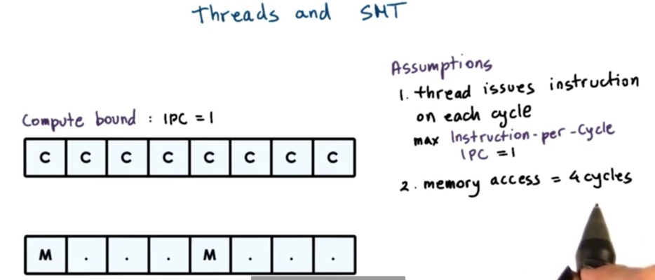
To understand what is required from a scheduler in a hyperthreaded platform we first need to make some assumptions.
First, we need to assume that a thread can issue an instruction on every CPU cycle. This means that a CPU bound thread will be able to maximize the instructions per cycle (IPC) metric.
Second, we need to assume that memory access takes four cycles. What this means is that a memory bound thread will experience some idle cycles while it is waiting for the memory access to complete.
Third, we can also assume that hardware switching is instantaneous.
Finally, we will assume that we have an SMT platform with two hardware threads.
Let's look at the scenario of co-scheduling two compute-bound threads.
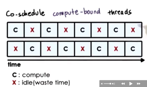
Even though each thread is able to issue a CPU instruction during each cycle, only one thread will be able to issue an instruction at a time since there is only one CPU pipeline. As a result, these threads will interfere with one another as they compete for CPU pipeline resources.
The best case scenario is that a thread idles every other cycle while it yields to the other thread issuing instructions. As a result, the performance of each thread degrades by a factor of two.
In addition, the memory component is completely idle during this computation, as nothing is performing any memory access.
Let's look at the scenario of co-scheduling two memory-bound threads.
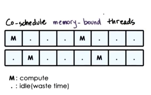
Similar to the CPU-bound thread example, we still have idle time where both threads are waiting on memory access to return, which means wasted CPU cycles.
Let's look at co-scheduling a mix of CPU and memory-bound threads.
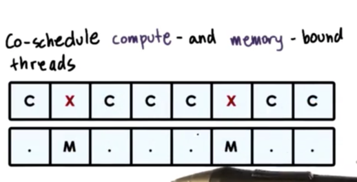
This solution seems best. We schedule the CPU-bound thread until the memory-bound thread needs to issue a memory request. We context switch over, issue the request, and then context switch back and continue our compute-heavy task. This way, we minimize the number of wasted CPU cycles.
Scheduling a mix of memory/CPU intensive threads allows us to avoid or at least limit the contention on the processor pipeline and helps to ensure utilization across both the CPU and the memory components.
Note that we will still experience some degradation due to the interference of these two threads, but it will be minimal relative to the co-scheduling of only memory- or CPU-bound threads.
CPU Bound or Memory Bound
How do we know if a thread is CPU bound or memory bound? We need to use historic information.
When we looked previously at determining whether a process was more interactive or more CPU intensive, we looked at the amount of time the process spent sleeping. This approach won't work in this case for two reasons. First of all, the thread is not really sleeping when it is waiting on memory access. It is waiting at some stage in the processor pipeline, not on some software queue. Second, to keep track of the sleep time we were using software methods and that is too slow at this level. The context switch takes on the order of cycles, so we need to be able to make our decision on what to run very quickly.
We need some hardware-level information in order to help make our decision.
Most modern platforms contain hardware counters that get updated as the processor executes and keep information about various aspects of execution, like
- L1, L2 … LLC cache misses
- Instructions Per Cycle (IPC) metrics
- Power/Energy usage data
There are a number of software interfaces for accessing these hardware counters, such as
- oprofile
- Linux perf tool
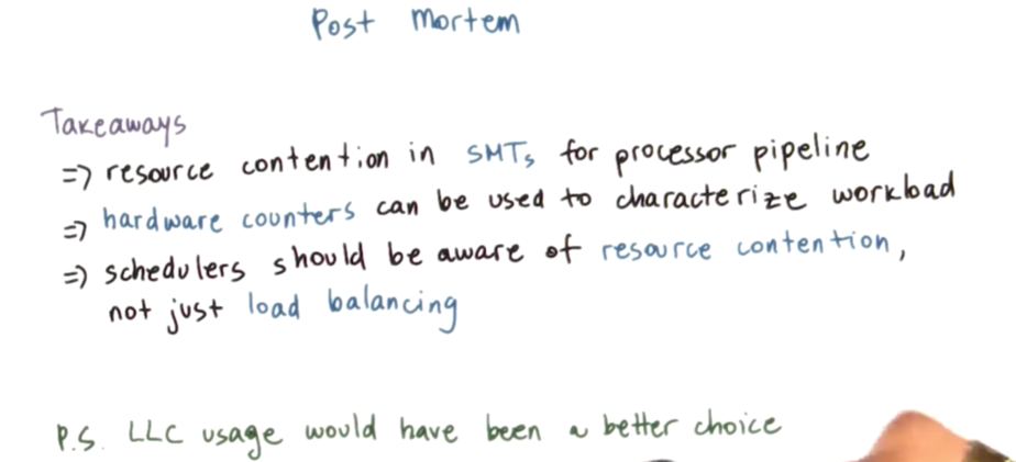
So how can hardware counters help us make scheduling decisions? Many practical scheduling techniques rely on the use of hardware counters to understand something about the resource needs of a thread. The scheduler can use this information to pick a good mix of the threads that are available in the runqueue to schedule in the system so that all of the components of the system are well utilized and the threads interfere with each other as little as possible.
For example, a thread scheduler can look at the number of LLC misses - a metric stored by the hardware counter - and determine that if this number is great enough then the thread is most likely memory bound.
Even though different hardware counters provide different metrics, schedulers can still make informed decisions from them. Schedulers often look at multiple counters across the CPU and can rely on models that have built for a specific platform and that have been trained using some well-understood workloads.
Scheduling with Hardware Counters
Fedorova speculates that a more concrete metric to help determine if a thread is CPU bound or memory bound is cycles per instruction (CPI). A memory bound thread will take a lot of cycles to complete an instruction; therefore, it has a high CPI. A CPU bound thread will have a CPI of 1 (or some low number) as it can complete an instruction every cycle (or close to every cycle).
Given that there is no CPI counter on the processor that Fedorova uses - and computing something like 1 / IPC would require unacceptable software intervention - she uses a simulator.
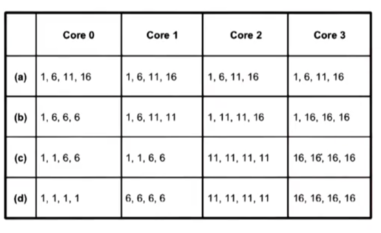
To explore this question, Fedorova simulates a system that has 4 cores, with each core have a 4-way SMT, for a total of 16 hardware execution contexts.
Next, she wants to vary the threads that get assigned to these hardware contexts based on their CPI, so she creates a synthetic workload where her threads have a CPI of 1, 6, 11, and 16. The threads with the CPI of 1 will be the most CPU-intensive, while the threads with the CPI of 16 will be the most memory-intensive. The overall workload mix has four threads of each kind.
She wants to assess is the overall performance when a specific mix of threads gets assigned to each of these 16 hardware contexts, and she uses IPC as the metric. Given that the maximum number of cores is 4, the maximum IPC is 4.
She runs four experiments, (a) - (d), with each core having a specific composition of threads.
CPI Experiment Results
Here are the results for the four experiments.
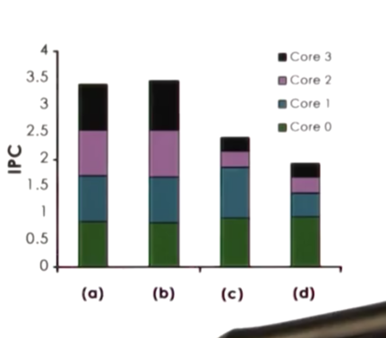
In the first two experiments, we have a fairly well balance mix of high- and low-CPI threads across the cores. We see that in these two cases, the processor pipeline was well-utilized and our IPC is high.
In the last two experiments, each of the cores were assigned tasks with similar - or in the case of the final experiment, identical - CPI values. We can see that in these two cases, the processor pipeline was much more poorly utilized. Threads either spent a lot of time in contention with one another - in the case of CPU bound tasks - or the CPU spent a lot of time idling - in the case of memory-bound tasks. Regardless, our IPC dropped significantly.
We can conclude that scheduling tasks with mixed CPI values leads to higher platform utilization.
We have used a synthetic workload in this case, with each task having a CPI that is quite far from other CPI values present in the system. Is this a realistic workload?
In order to answer this, Fedorova profiled a number of applications from several respected benchmark suites and computed the CPI values for each.
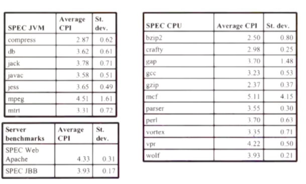
What we can see is that most of the values are quite cluttered together. We do not see the distinct values presented in the synthetic workload. Most CPIs range from 2.5 - 4.5.
Because CPI isn't that different across applications, it may not be the most instructive metric to inform scheduling decisions.
OMSCS Notes is made with in NYC by Matt Schlenker.
Copyright © 2019-2023. All rights reserved.
privacy policy