Computer Networks
Transport and Application Layers
31 minute read
Notice a tyop typo? Please submit an issue or open a PR.
Transport and Application Layers
Introduction to Transport Layer and the Relationship between Transport and Network Layer
The transport layer provides an end-to-end connection between two applications that are running on different hosts. Of course the transport layer provides this logical connection regardless if the hosts are in the same network.
Here is how it works; The transport layer on the sender host receives a message from the application layer and it appends its own header. We refer to this combined message as a segment. This transport layer segment is then sent to the network layer which will further append (encapsulate) this segment with its header information. Then it will send it to the receiving host via routers, bridges, switches etc.
One might ask, why do we need an additional layer between the application and the network layer? Recall, that the network-layer is based on a best effort delivery service model. According to this model, the network layer makes a best effort to deliver data packets. Thus, it doesn't guarantee the delivery of packets, nor it guarantees integrity in data. So, here is where the transport layer comes to offer some of these functionalities. This allows application programmers to develop applications assuming a standard set of functionalities that are provided by the transport layer. So the applications can run over diverse networks without having to worry about different network interfaces or possible unreliability of the network.
Within the transport layer, there are two main protocols: User datagram protocol (UDP) and the Transmission Control Protocol (TCP). These protocols differ based on the functionality they offer to the application developers; UDP provides very basic functionality and relies on the application-layer to implement the remaining. On the other hand, TCP provides some strong primitives with a goal to make end-to-end communication more reliable and cost-effective. In fact, because of these primitives, TCP has become quite ubiquitous and is used for most of the applications today. We will now look at these functionalities in detail.
Multiplexing: why we need it?
One of the main desired functionalities of the transport layer is the ability for a host to run multiple applications to use the network simultaneously; which we refer to as multiplexing.
Let us consider a simple example to further illustrate why we need transport-layer multiplexing. Consider a user who is using Facebook while also listening to music on Spotify. Clearly, both of these processes involve communication to two different servers. How do we make sure that the incoming packets are delivered to the correct application? Note that, the network layer uses only the IP address and an IP address alone does not say anything about which processes on the host should get the packets. Thus, we need an addressing mechanism to distinguish the many processes sharing the same IP address on the same host.
The transport layer solves this problem, by using additional identifiers known as ports. Each application binds itself to a unique port number by opening sockets and listening for any data from a remote application. Thus, the transport layer can do multiplexing by using ports.
There are two ways in which we can use multiplexing. Connectionless and connection oriented multiplexing. As the name suggests, it depends if we have a connection established between the sender and the receiver or not.
In the next topic we are looking into multiplexing and demultiplexing.
Connection Oriented and Connectionless Multiplexing and Demultiplexing
In this topic, we will talk about multiplexing and demultiplexing.
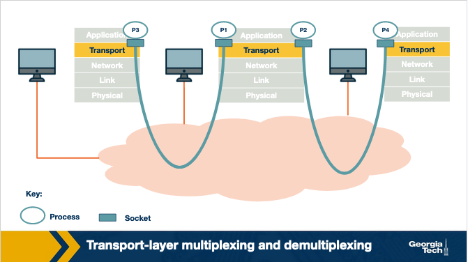
Let's consider the scenario shown in the figure above which includes three hosts running an application. A receiving host that receives an incoming transport-layer segment will forward it to the appropriate socket. The receiving host identifies the appropriate socket by examining a set of fields in the segment.
The job of delivering the data that are included in a transport-layer segment to the appropriate socket, as defined in the segment fields, is called demultiplexing.
Similarly, the sending host will need to gather data from different sockets, and encapsulate each data chunk with header information (that will later be used in demultiplexing) to create segments, and then forward the segments to the network layer. We refer to this job as multiplexing.
As an example, let's take a closer look at the host in the middle. The transport layer in the middle host, will need to demultiplex the data arriving from the network layer to the correct socket (P1 or P2). Also, the transport layer in the middle host, will need to perform multiplexing, by collecting the data from sockets P1 or P2, then by generating transport-layer segments, and then finally by forwarding these segments to the network layer below.
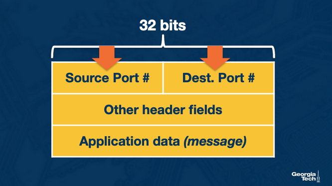
Now, let's focus at the socket identifiers: The sockets are identified based on special fields (shown below) in the segment such as the source port number field and the destination port number field.
We have two flavors of multiplexing/demultiplexing: the connectionless and connection oriented.
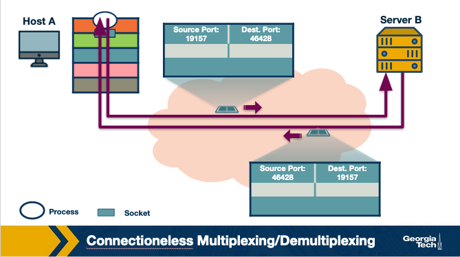
First, we will talk about the connectionless multiplexing and demultiplexing. The identifier of a UDP socket is a two-tuple that is consisted of a destination IP address and a destination port number. Consider two hosts, A and B, which are running two processes at UDP ports a and b respectively. Let's suppose that host A sends data to host B. The transport layer in host A creates transport layer segment by the application data, the source port and the destination port, and forwards the segment to the network layer. In turn the network layer encapsulates the segment into a network-layer datagram and sends it to host B with best effort delivery. Let's suppose that the datagram is successfully received by host B. Then the transport layer at host B, identifies the correct socket by looking at the field of the destination port. In case that host B runs multiple processes, each process will have its own own UDP socket and therefore a distinct associated port number. Host B will use this information to demultiplex receiving data to the correct socket. If Host B receives UDP segments with destination port number, it will forward the segments to the same destination process via the same destination socket, even if the segments are coming from different source hosts and/or different source port numbers.
Now let's consider the connection oriented multiplexing and demultiplexing.
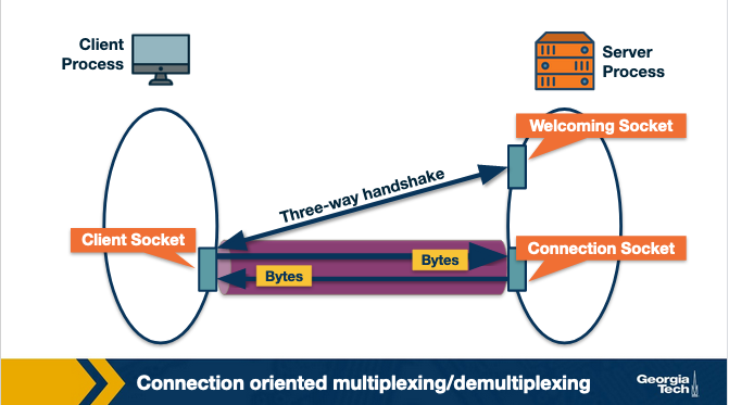
The identifier for a TCP socket is a four tuple that is consisted by the source IP, source port, destination IP and destination port. Let's consider the example of a TCP client server as shown in the figure 2.29. The TCP server has a listening socket that waits for connections requests coming from TCP clients. A TCP client creates a socket and sends a connection request, which is a TCP segment that has a source port number chosen by the client, a destination port number 12000 and a special connection-establishment bit set in the TCP header. Finally, the TCP server receives the connection request, and the server creates a socket that is identified by the four-tuple source IP, source port, destination IP and destination port. The server uses this socket identifier to demultiplex incoming data and forward them to this socket. Now, the TCP connection is established and the client and server can send and receive data between one another.
Example: Let's look at an example connection establishment.
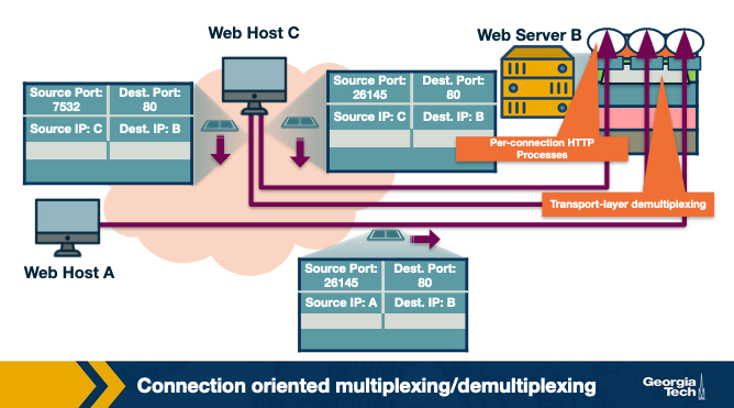
In this example, we have three hosts A, B and C. Host C and A initiate two and one HTTP sessions to server B, respectively. Hosts C and A assign port numbers to their connections independently of one another. Host C assigns port numbers 26145 and 7532. In case Host A assigns the same port number as C, host B will still be able to demultiplex incoming data from the two connections because the connections are associated with different source IP addresses.
Let's add a final note about web servers and persistent HTTP. Let's assume, we have a webserver listening for connection requests at port 80. Clients send their initial connection requests and their subsequent data with destination port 80. The webserver is able to demultiplex incoming data based on their unique source IP addresses and source port numbers. The client and the server maybe persistent HTTP, in which case, they exchange HTTP messages via the same server socket. The client and the server maybe using non-persistent HTTP, where for every request and response, a new TCP connection and a new socket are created and closed for every response/request. In the second case, a busy webserver may experience severe performance impact.
As we have seen, UDP and TCP use port numbers to identify the sending application and destination application. Why don't UDP and TCP just use process IDs rather than define port numbers?
Process IDs are specific to operating systems and therefore using process IDs rather than a specially defined port would make the protocol operating system dependent. Also, a single process can set up multiple channels of communications and so using the process ID as the destination identifier wouldn't be able to properly demultiplex, Finally, having processes listen on well-known ports (like 80 for http) is an important convention.
A word about the UDP protocol
This lecture is primarily focused on TCP. Before exploring more topics on the TCP protocol let's briefly talk about UDP.
UDP is: a) an unreliable protocol as it lacks the mechanisms that TCP has in place and b) a connectionless protocol that does not require the establishment of a connection (e.g. threeway handshake) before sending packets.
The above description doesn't sound so promising... so why do we have UDP at the first place? Well, it turns out that it is exactly the lack of those mechanisms that make UDP more desirable in some cases.
Specifically UDP offers less delays and better control over sending data because with UDP we have:
- No congestion control or similar mechanisms. With UDP, as soon as the application passes data to the transport layer, then UDP encapsulates it and sends it over to the network layer. In contrast TCP “intervenes” a lot with sending the data (e.g. with the congestion control mechanism or the retransmissions in case an ACK is not received). These TCP mechanisms cause further delays.
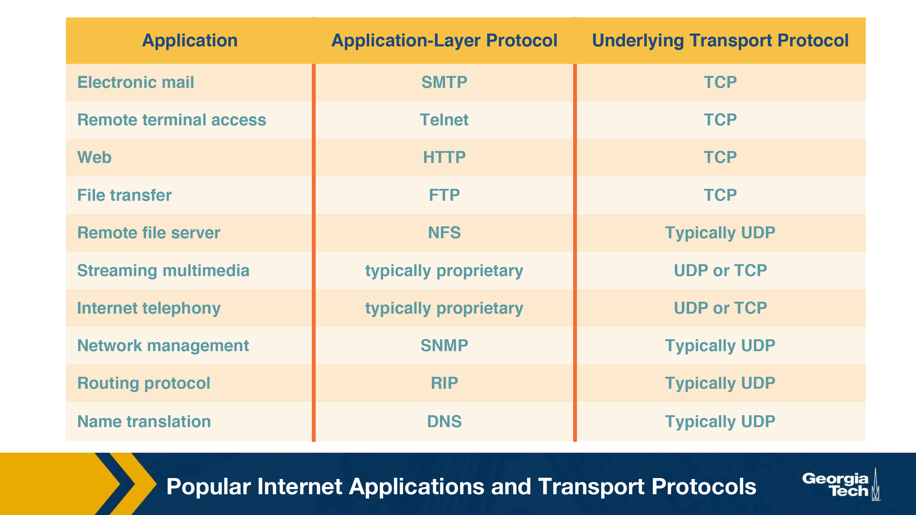
- No connection management overhead. With UDP we have no connection establishment and no need to keep track of connection state (e.g. with buffers). Both mean even less delays. So with some real time applications that are sensitive to delays UDP is a better option, despite possibly higher losses (e.g. DNS is using UDP). Which other applications prefer UDP over TCP? The table below gives us an idea:
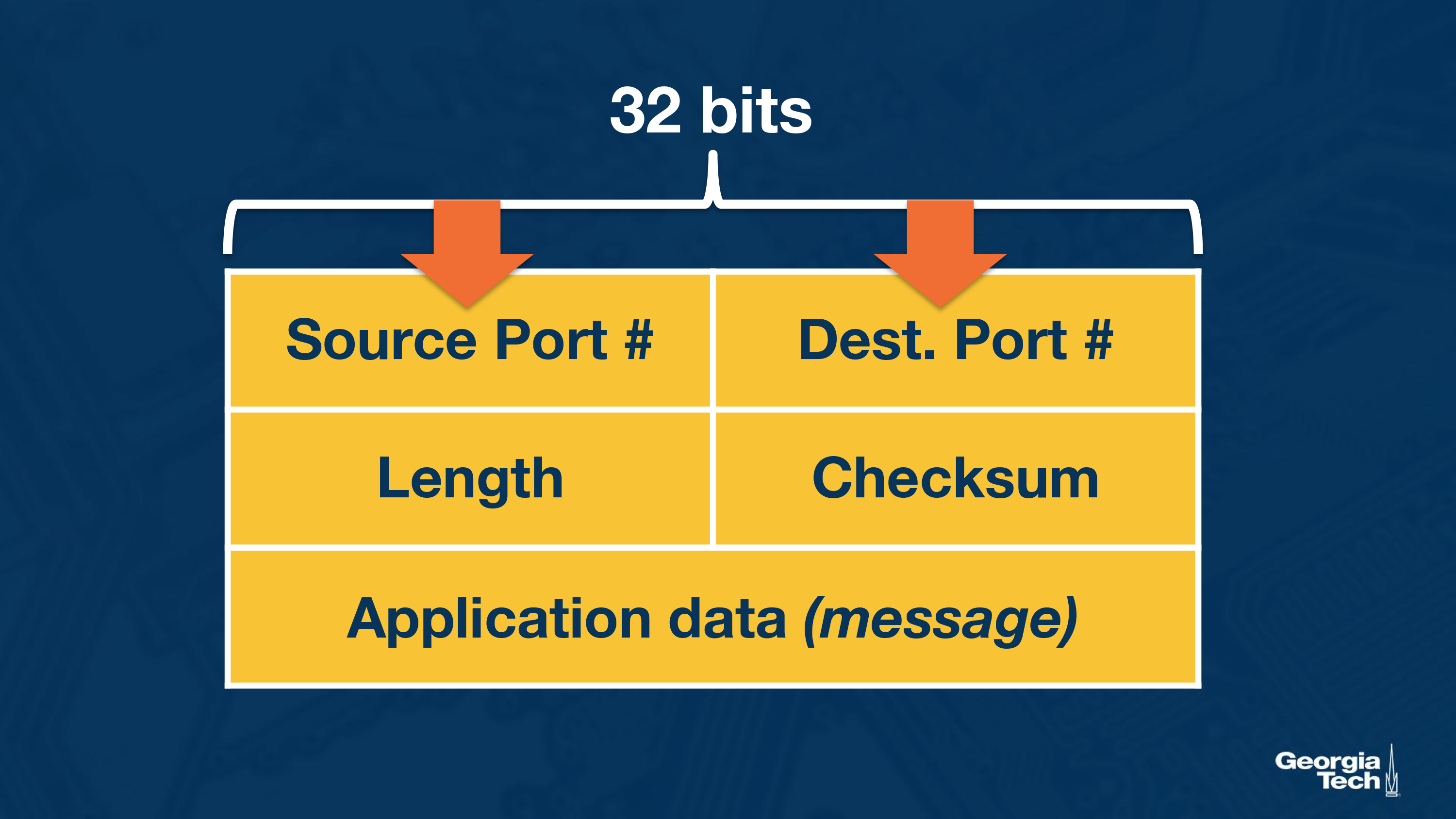
The UDP packet structure: UDP has a 64 bits header consisting of the following fields:
- Source and destination ports.
- Length of the UDP segment (header and data).
- Checksum (an error checking mechanism). Since there is no guarantee for link-by-link reliability, we need a basis mechanism in place for error checking. The UDP sender adds the src port, the dest port and the packet length. Then it takes the sum and performs an 1s complement (all 0s are turned to 1 and all 1s are turned to 0s). If during the sum there is an overflow, its wrapped around. The receiver adds all the four 16-bit words (including the checksum). The result should be all 1s unless an error has occurred.
UDP and TCP use 1's complement for their checksums. But why is it that UDP takes the 1's complement of the sum – why not just use the sum? Exploring this further, using 1's complement, how does the receiver compute and detect errors? Using 1's complement, is it possible that a 1-bit error will go undetected? What about a 2-bit error?
To detect errors, the receiver adds the four words (the three original words and the checksum). If the sum contains a zero, the receiver knows there has been an error. While all one-bit errors will be detected, but two-bit errors can be undetected (e.g., if the last digit of the first word is converted to a 0 and the last digit of the second word is converted to a 1).
The TCP Three-Way Handshake
The TCP Three way Handshake
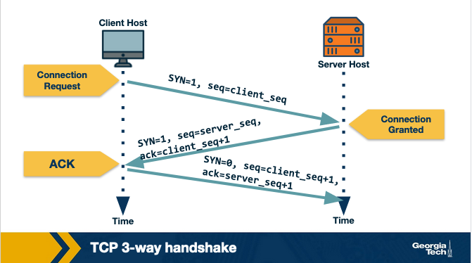
Step 1: The TCP client sends a special segment, (containing no data) and with SYN bit set to 1. The Client also generates an initial sequence number (client_isn) and includes it in this special TCP SYN segment.
Step 2: The Server upon receiving this packet, allocates the required resources for the connection and sends back the special ‘connection-granted' segment which we call SYNACK. This packet has SYN bit set to 1, ack field containing (client_isn+1) value and a randomly chosen initial sequence number in the sequence number field.
Step 3: When the client receives the SYNACK segment, it also allocates buffer and resources for the connection and sends an acknowledgment with SYN bit set to 0.
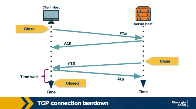
Connection Teardown
Step 1: When client wants to end the connection, it sends a segment with FIN bit set to 1 to the server.
Step 2: Server acknowledges that it has received the connection closing request and is now working on closing the connection.
Step 3: The Server then sends a segment with FIN bit set to 1, indicating that connection is closed.
Step 4: The Client sends an ACK for it to the server. It also waits for sometime to resend this acknowledgment in case the first ACK segment is lost.
Reliable Transmission
What is reliable transmission? Recall that the network layer is unreliable and it may lead to packets getting lost or arriving out of order. This can clearly be an issue for a lot of applications. For example, a file downloaded over the Internet might be corrupted if some of the packets were lost during the transfer.
One option here is to allow the application developers take care of the network losses as is done in UDP. However, given that reliability is an important primitive desirable for a lot of applications, TCP developers decided to implement this primitive in the transport layer. Thus, TCP guarantees an in-order delivery of the application-layer data without any loss or corruption.
Now, let us look at how TCP implements reliability.
In order to have a reliable communication, the sender should be able to know which segments were received by the remote host and which were lost. Now, how can we achieve this? One way to do this is by having the receiver send acknowledgements indicating that it has successfully received the specific segment. In case the sender does not receive an acknowledgement within a given period of time, the sender can assume the packet is lost and resend it. This method of using acknowledgements and timeouts is also known as Automatic Repeat Request or ARQ.
There are various methods in which it can be implemented:
The simplest way would be for the sender to send a packet and wait for its acknowledgement from the receiver. This is known as Stop and Wait ARQ. Note that the algorithm typically needs to figure out the waiting time after which it resends the packet and this estimation can be tricky. A small value of timeout can lead to unnecessary re-transmissions and a large value can lead to unnecessary delays. In most cases, the timeout value is a function of the estimated round trip time of the connection.
Clearly, this kind of alternate sending and waiting for acknowledgement has a very low performance. In order to solve this problem, the sender can send multiple packets without waiting for acknowledgements. More specifically, the sender is allowed to send at most N unacknowledged packets typically referred to as the window size. As it receives acknowledgement from the receiver, it is allowed to send more packets based on the window size. In implementing this, we need to take care of the following concerns:
- The receiver needs to be able to identify and notify the sender of a missing packet. Thus, each packet is tagged with a unique byte sequence number which is increased for subsequent packets in the flow based on the size of the packet.
- Also, now both sender and receiver would need to buffer more than one packet. For instance, the sender would need to buffer packets that have been transmitted but not acknowledged. Similarly, the receiver may need to buffer the packets because the rate of consuming these packets (say writing to a disk) is slower than the rate at which packets arrive.
Now let's look at how does the receiver notify the sender of a missing segment.
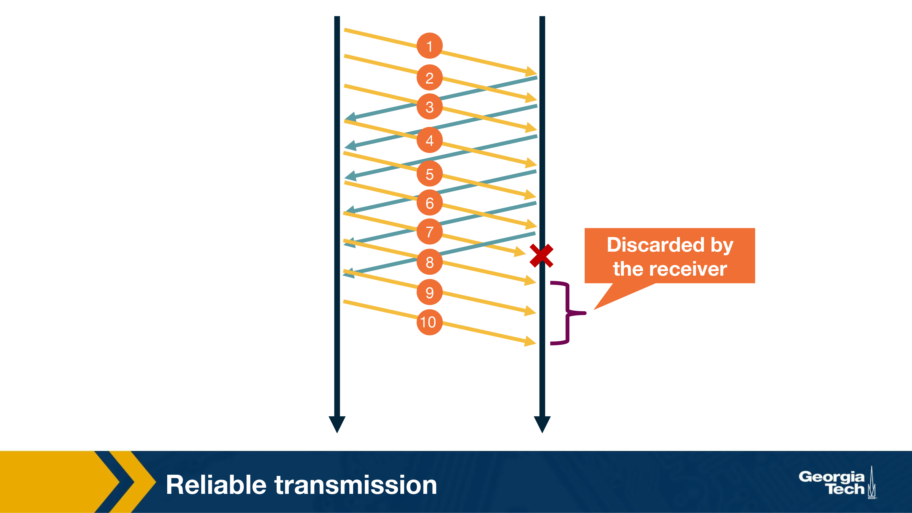
One way is for the receiver to send an ACK for the most recently received in-order packet. The sender would then send all packets from the most recently received in-order packet, even if some of them had been sent before. The receiver can simply discard any out-of-order received packets. This is called Go-back-N. For instance, in the figure below if packet 7 was lost in the network, the receiver will discard any subsequent packets. The sender will send all the packets starting from 7 again.
Clearly, in the above case, a single packet error can cause a lot of unnecessary retransmissions. To solve this, TCP uses selective ACKing. In this, the sender retransmits only those packets that it suspects were received in error. The receiver in this case would acknowledge a correctly received packet even if it is not in order. The out-of-order packets are buffered until any missing packets have been received at which point the batch of the packets can be delivered to the application layer.
Note that even in this case, TCP would need to use a timeout as there is a possibility of ACKs getting lost in the network.
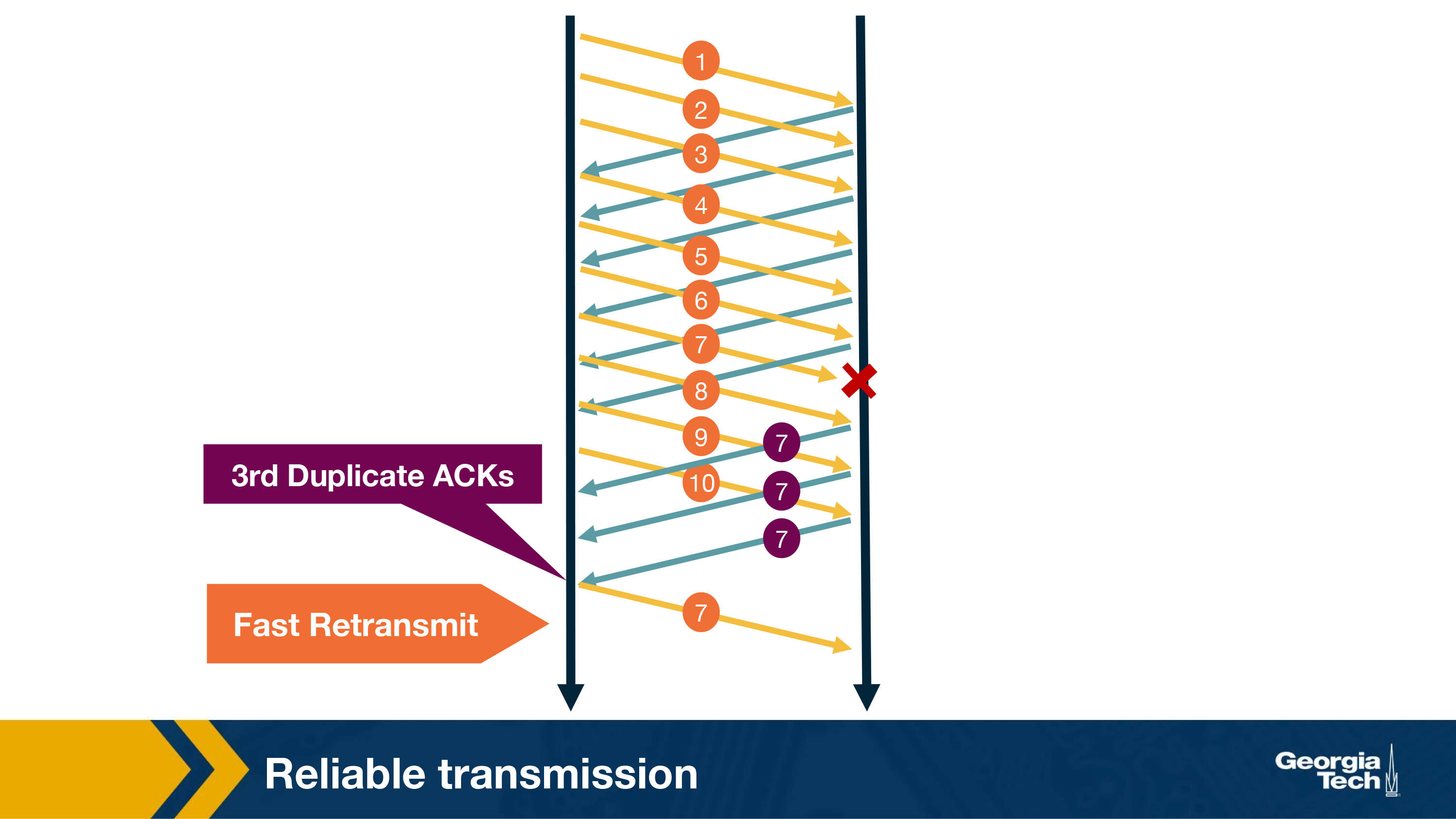
In addition to using timeout to detect loss of packets, TCP also uses duplicate acknowledgements as a means to detect loss. A duplicate ACK is additional acknowledgement of a segment for which the sender has already received acknowledgment earlier. When the sender receives 3 duplicate ACKs for a packet, it considers the packet to be lost and will retransmit it instead of waiting for the timeout. This is known as fast retransmit. For example, in the figure below, once sender receives 3 duplicate ACKs, it will retransmit packet 7 without waiting for timeout.
Transmission Control
In this topic we will learn about the mechanisms provided in the transport-layer to control the transmission rate.
Why control the transmission rate? We will first illustrate why we need to know and adapt the transmission rate. Consider a scenario when user A needs to send 1 Gb of file to a remote host B on a 100 Mbps link. What rate should it send the file? One could say that it should be 100 Mbps. But how does user A determine that given it does not know the link capacity. Also, what about other users that also would be using the same link? What happens to the sending rate if the receiver B is also receiving files from a lot of other users? Finally, which layer in the network decides the data transmission rate? In this section, we will try to answer all these questions.
Where should the transmission control function reside in the network stack? One option is to let the application developers figure out and implement mechanisms for transmission control. This is what UDP does. However, it turns out that transmission control is a fundamental function for most of the applications. Thus it will be easier if it is implemented in the transport layer. Moreover, it also has to deal with issues of fairness in using the network as we will see later, thus making it more convenient to handle it at the transport layer. Thus, TCP provides mechanisms for transmission control which have been a subject of interest to network researchers since the inception of computer networking. We will look at these in detail now.
Flow Control
Flow control: Controlling the transmission rate to protect the receiver's buffer
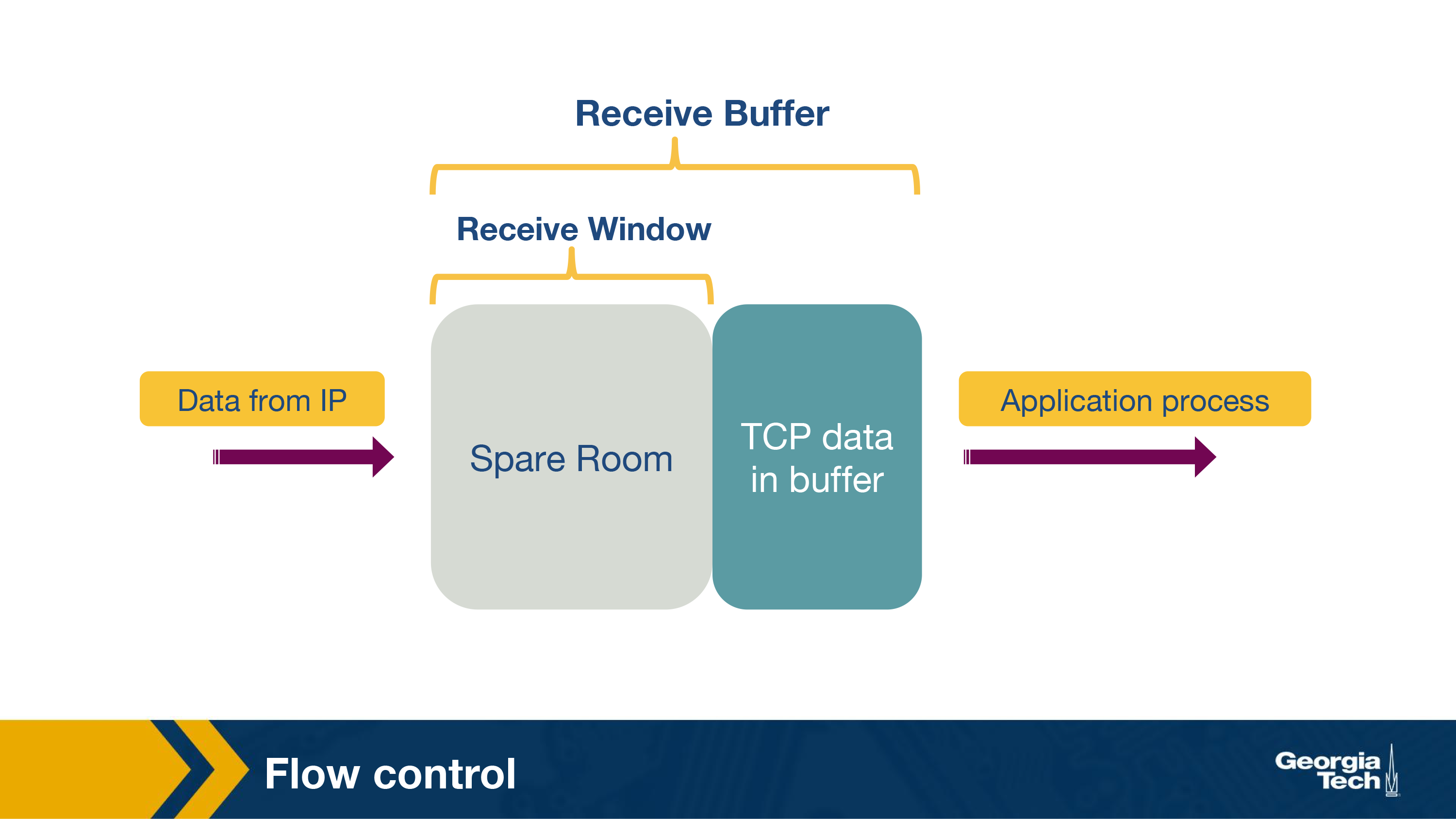
The first case where we need transmission control is to protect the buffer of the receiver from overflowing. Recall that TCP uses a buffer at the receiver end to buffer packets that have not been transmitted to the application. It could happen that the receiver is involved with multiple processes and does not read the data instantly. This can cause accumulation of huge amount of data and overflow the receive buffer.
TCP provides a rate control mechanism also known as flow control that helps match the sender's rate against the receiver's rate of reading the data. Sender maintains a variable ‘receive window'. It provides sender an idea of how much data the receiver can handle at the moment.
We will illustrate its working using an example. Consider two hosts, A and B, that are communicating with each other over a TCP connection. Host A wants to send a file to Host B. For this, Host B allocates a receive buffer of size RcvBuffer to this connection. The receiving host maintains two variables, LastByteRead (number of byte that was last read from the buffer ) and LastByteRcvd (last byte number that has arrived from sender and placed in the buffer). Thus, in order to not overflow the buffer, TCP needs to make sure that
LastByteRcvd - LastByteRead <= RcvBuffer
The extra space that the receive buffer has, is specified using a parameter, termed as receive window.
rwnd = RcvBuffer - [LastByteRcvd - LastByteRead]
The receiver advertises this value of rwnd in every segment/ACK it sends back to the sender.
The sender also keeps track of two variables, LastByteSent and LastByteAcked.
UnAcked Data Sent = LastByteSent - LastByteAcked
To not overflow the receiver's buffer, the sender needs to make sure that the maximum number of unacknowledged bytes it sends are no more than the rwnd.
Thus we need:
LastByteSent - LastByteAcked <= rwnd
Caveat: However, there is one scenario where this scheme has a problem. Consider a scenario, if the receiver had informed the sender that rwnd = 0, and thus the sender stops sending data. Also, assume that B has nothing to send to A. Now, as the application processes the data at the receiver, the receiver buffer is cleared but the sender may never know that new buffer space is now available and will be blocked from sending data even when receiver buffer is empty.
TCP resolves this problem by making sender continue sending segments of size 1 byte even after when rwnd = 0. When the receiver acknowledges these segments, it will specify the rwnd value and the sender will know as soon as the receiver has some room in the buffer.
Congestion Control Introduction
Congestion control: Controlling the transmission rate to protect the network from congestion
The second and very important reason for transmission control is to avoid congestion in the network.
Let us look at an example to understand this. Consider a set of senders and receivers sharing a single link with capacity C. Assume, other links have capacity > C. How fast should each sender transmit data? Clearly, we do not want the combined transmission rate to be higher than the capacity of the link as it can cause issues in the network such as longer queues, packet drops etc. Thus, we want a mechanism to control the transmission rate at the sender in order to avoid congestion in the network. This is known as congestion control.
It is important to note that networks are quite dynamic with users joining and leaving the network, initiating data transmission and terminating existing flows. Thus the mechanisms for congestion control need to be dynamic enough to adapt to these changing network conditions.
What are the goals of congestion control?
Let us consider some of the desirable properties of a good congestion control algorithm:
- Efficiency: We should get high throughput or utilization of the network should be high.
- Fairness: Each user should its fair share of the network bandwidth. The notion of fairness is dependent on the network policy. For this context, we will assume that every flow under the same bottleneck link should get equal bandwidth.
- Low delay: In theory, it is possible to design protocols that have consistently high throughput assuming infinite buffer. Essentially, we could just keep sending the packets to the network and they will get stored in the buffer and will eventually get delivered. However, it will lead to long queues in the network leading to delays. Thus, applications that are sensitive to network delays such as video conferencing will suffer. Thus, we want the network delays to be small.
- Fast convergence: The idea here is that a flow should be able to converge to its fair allocation fast. This is important as a typical network's workload is composed a lot of short flows and few long flows. If the convergence to fair share is not fast enough, the network will still be unfair for these short flows.
Congestion control flavors: E2E vs Network-assisted
Broadly speaking, there can be two approaches to implement congestion control:
The first approach is network-assisted congestion control. In this we rely on the network layer to provide explicit feedback to the sender about congestion in the network. For instance, routers could use ICMP source quench to notify the source that the network is congested. However, under severe congestion, even the ICMP packets could be lost, rendering the network feedback ineffective.
The second approach is to implement end-to-end congestion control. As opposed to the previous approach, the network here does not provide any explicit feedback about congestion to the end hosts. Instead, the hosts infer congestion from the network behavior and adapt the transmission rate.
Eventually, TCP ended up using the end-to-end approach. This largely aligns with the end-to-end principle adopted in the design of the networks. Congestion control is a primitive provided in the transport layer, whereas routers operate at the network layer. Therefore, the feature resides in the end nodes with no support from the network. Note that this is no longer true as certain routers in the modern networks can provide explicit feedback to the end-host by using protocols such as ECN and QCN.
Let us now look at how TCP can infer congestion from the behavior of the network.
How a host infers congestion? Signs of congestion
There are mainly two signals of congestion.
First is the packet delay. As the network gets congested, the queues in the router buffers build up. This leads to increased packet delays. Thus, an increase in the round trip time, which can be estimated based on ACKs, can be an indicator of congestion in the network. However, it turns out that packet delay in a network tend to be variable, making delay-based congestion inference quite tricky.
Another signal for congestion is packet loss. As the network gets congested, routers start dropping packets. Note that packets can also be lost due to other reasons such as routing errors, hardware failure, TTL expiry, error in the links, or flow control problems, although it is rare.
The earliest implementation of TCP ended up using loss as a signal for congestion. This is mainly because TCP was already detecting and handling packet losses to provide reliability.
How does a TCP sender limit the sending rate?
The idea of TCP congestion control was introduced so that each source can determine the network's available capacity and know how many packets it can send without adding to the network's level of congestion. Each source uses ACKs as a pacing mechanism. Each source uses the ACK to determine if the packet released earlier to the network was received by the receiving host and it is now safe to release more packets into the network.
TCP uses a congestion window which is similar to the receive window used for flow control. It represents the maximum number of unacknowledged data that a sending host can have in transit (sent but not yet acknowledged).
TCP uses a probe-and-adapt approach in adapting the congestion window. Under regular conditions, TCP increases the congestion window trying to achieve the available throughput. Once it detects congestion then the congestion window is decreased.
In the end, the number of unacknowledged data that a sender can have is the minimum of the congestion window and the receive window.
LastByteSent - LastByteAcked <= min{cwnd, rwnd}
In a nutshell, a TCP sender cannot send faster than the slowest component, which is either the network or the receiving host.
Congestion control at TCP - AIMD
TCP decreases the window when the level of congestion goes up, and it increases the window when the level of congestion goes down. We refer to this combined mechanism as additive increase/multiplicative decrease (AIMD).
Additive Increase
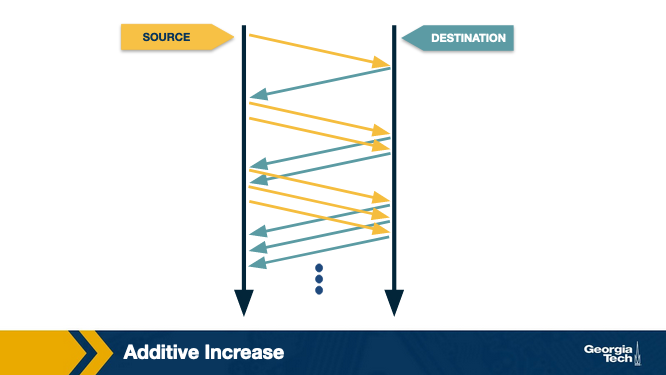
The connection starts with a constant initial window, typically 2 and increases it additively. The idea behind additive increase is to increase the window by one packet every RTT (Round Trip Time). So, in the additive increase part of the AIMD, every time the sending host successfully sends a cwnd number of packets it adds 1 packet to cwnd.
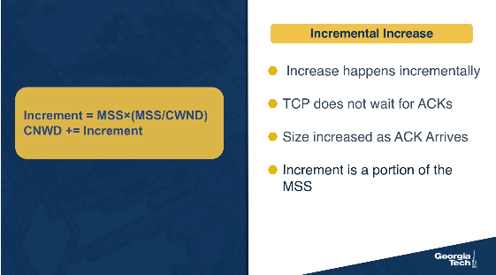
Also, in practice, this increase in AIMD happens incrementally. TCP doesn't wait for ACKs of all the packets from the previous RTT. Instead, it increases the congestion window size as soon as each ACK arrives. In bytes, this increment is a portion of the MSS (Maximum Segment Size).
Increment = MSS × (MSS / CongestionWindow)
CongestionWindow += Increment
Multiplicative Decrease
Once TCP Reno detects congestion, it reduces the rate at which the sender transmits. So, when the TCP sender detects that a timeout occurred, then it sets the CongestionWindow (cwnd) to half of its previous value. This decrease of the cwnd for each timeout corresponds to the “multiplicative decrease” part of AIMD. For example, suppose the cwnd is currently set to 16 packets. If a loss is detected, then cwnd is set to 8. Further losses would result to the cwnd to be reduced to 4 and then to 2 and then to 1. The value of cwnd cannot be reduce further than 1 packet.
Figure below shows an example of how the congestion control window decreases when congestion is detected:
Signals of congestion
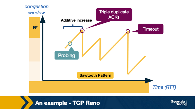
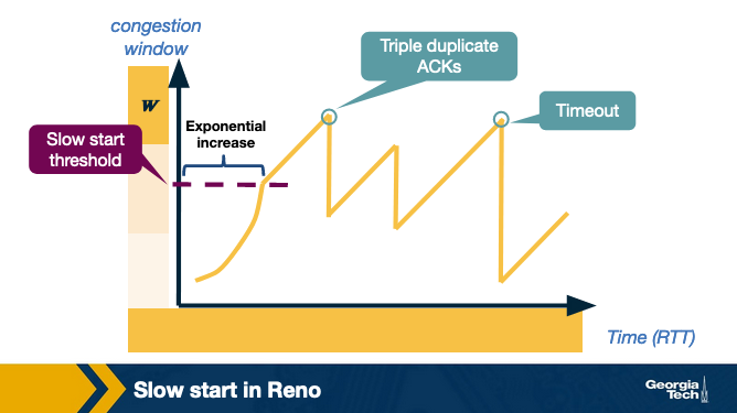
TCP Reno uses two types of packet loss detection as a signal of congestion. First is the triple duplicate ACKs and is considered to be mild congestion. In this case, the congestion window is reduced to half of the original congestion window.
The second kind of congestion detection is timeout i.e. when no ACK is received within a specified amount of time. It is considered a more severe form of congestion, and the congestion window is reset to the Initial Window.
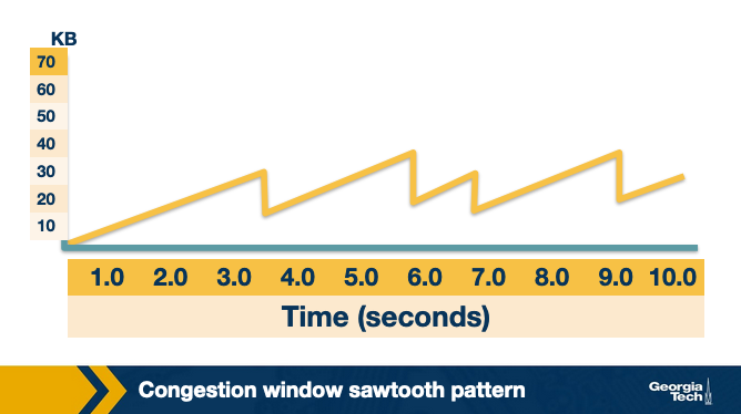
Congestion window sawtooth pattern
TCP continually decreases and increases the congestion window throughout the lifetime of the connection. If we plot the cwnd with respect to time, we observe that it follows a sawtooth pattern as shown in the figure:
Slow start in TCP
The AIMD approach we saw in the previous topic is useful when the sending host is operating very close to the network capacity. AIMD approach reduces the congestion window at a much faster rate than it increases the congestion window. The main reason for this approach is that the consequences of having too large a window are much worse than those of it being too small. For example, when the window is too large, more packets will be dropped and retransmitted, making network congestion even worse; thus, it is important to reduce the number of packets being sent into the network as quickly as possible.
In contrast, when we have a new connection that starts from cold start, it can take much longer for the sending host to increase the congestion window by using AIMD. So for a new connection, we need a mechanism which can rapidly increase the congestion window from a cold start.
To handle this, TCP Reno has a slow start phase where the congestion window is increased exponentially instead of linearly as in the case of AIMD. The source host starts by setting cwnd to 1 packet. When it receives the ACK for this packet, it adds 1 to the current cwnd and sends 2 packets. Now when it receives the ACK for these two packets, it adds 1 to cwnd for each of the ACK it receives and sends 4 packets. Once the congestion window becomes more than a threshold, often referred to as slow start threshold, it starts using AIMD.
The figure below shows the sending host during slow start.
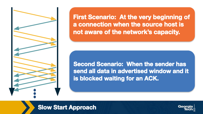
The figure below shows an example of the slow start phase.
Slow start is called “slow” start despite using an exponential increase because in the beginning it sends only one packet and starts doubling it after each RTT. Thus, it is slower than starting with a large window.
Finally, we note that there is one more scenario, where slow start kicks in. When a connection dies while waiting for a timeout to occur. This happens when the source has sent enough data as allowed by the flow control mechanism of TCP and times out while waiting for the ACK which will not arrive. Thus, the source will eventually receive a cumulative ACK that will reopen the connection and then instead of sending the available window size worth of packets at once, it will use slow start mechanism.
In this case, the source will have a fair idea about the congestion window from the last time it had a packet loss. It will now use this information as the “target” value to avoid packet loss in future. This target value is stored in a temporary variable “CongestionThreshold”. Now, source performs slow start by doubling the number of packets after each RTT until cwnd value reaches the congestion threshold (a knee point). After this point, it increases the window by 1 (additive increase) each RTT until it experiences packet loss (cliff point). After which it multiplicatively decreases the window.
TCP Fairness
Recall that we defined fairness as one of the desirable goals of congestion control. Note that fairness in this case means that for k-connections passing through one common link with capacity R bps, each connection gets an average throughput of R/k.
Let us understand if TCP is fair.
Consider a simple scenario where two TCP connections share a single link with bandwidth R. For simplicity, we assume that both connections have same RTT and there are only TCP segments passing through the link. If we plot a graph for throughput of these two connections, then the throughput for each should sum up to R. So, the goal is to get throughput achieved for each link fall somewhere near the intersection of the equal bandwidth share line and the full bandwidth utilization line, as shown in below graph:
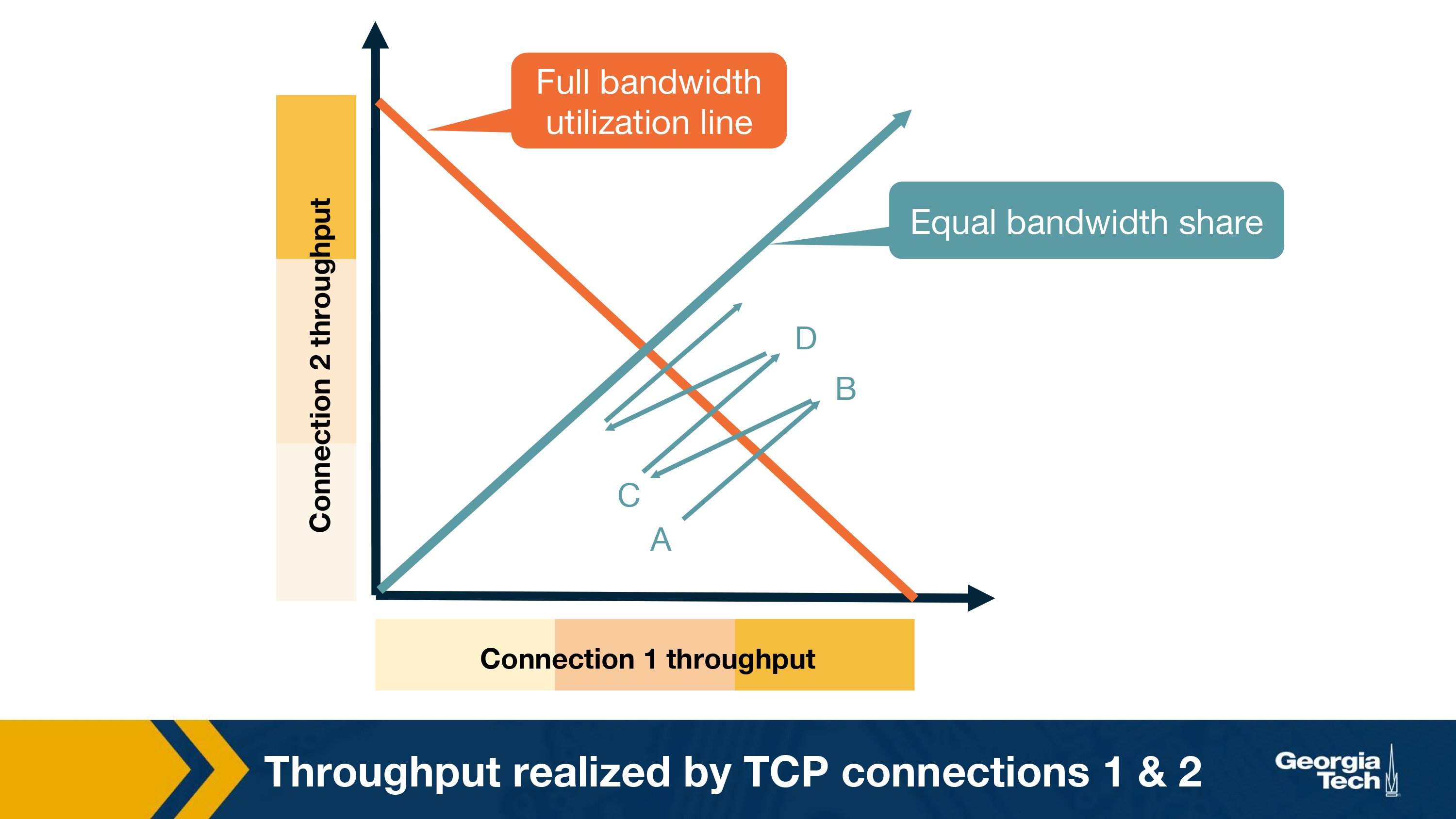
At point A in the above graph, total utilized bandwidth is less than R, so no loss can occur at this point. Therefore, both the connection will increase their window size, thus the sum of the utilized bandwidth will grow and graph will move towards B.
At point B, as the total transmission rate is more than R, both connection may start having packet loss. Now they will decrease their window size to half and come back to point C.
At point C, again the total throughput is less than R, so both connection will increase their window size to move towards point D and will again experience packet loss at D, and so on.
Thus, using AIMD leads to fairness in bandwidth sharing.
TCP utilizes the Additive Increase Multiplicative Decrease (AIMD) policy for fairness. Consider other possible policies for fairness in congestion control would be Additive Increase Additive Decrease (AIAD), Multiplicative Increase Additive Decrease (MIAD), and Multiplicative Increase Multiplicative Decrease (MIMD).
In AIAD and MIMD, the hosts communicating over the network will oscillate along the efficiency line, but will not converge as was shown for AIMD. MIAD will converge just like AIMD. But none of the alternative policies are as stable. The decrease policy in AIAD and MIAD is not as aggressive by comparison to AIMD and won't address congestion control as effectively. The increase policy in MIAD and MIMD is too aggressive.
Caution about fairness
There can be cases when TCP is not fair.
One such case arises due to the difference in the RTT of different TCP connections. Recall that TCP Reno uses ACK-based adaptation of the congestion window. Thus, connections with smaller RTT values would increase their congestion window faster than the ones with longer RTT values. This leads to an unequal sharing of the bandwidth.
Another case of unfairness arises if a single application uses multiple parallel TCP connections. Consider, for example, nine applications using one TCP connection sharing a link of rate R. If a new application establishes connection on the same link and also uses one TCP connection, then each application gets fairly the same transmission rate of R/10. But if the new application had 11 parallel TCP connections, then it would get an unfair allocation of more than R/2.
Congestion Control in Modern Network Environments: TCP CUBIC
Over the years, networks have improved with link speeds increasing tremendously. This has called for changes in the TCP congestion control mechanisms mainly with a desire to improve link utilization.
We can see that TCP Reno has low network utilization, especially when the network bandwidth is high or the delay is large. Such networks are also known as high bandwidth delay product networks.
To make TCP more efficient under such networks, many improvements to TCP congestion control have been proposed. Now we will look at one such version, called TCP CUBIC, which was also implemented in the Linux kernel. It uses a CUBIC polynomial as the growth function.
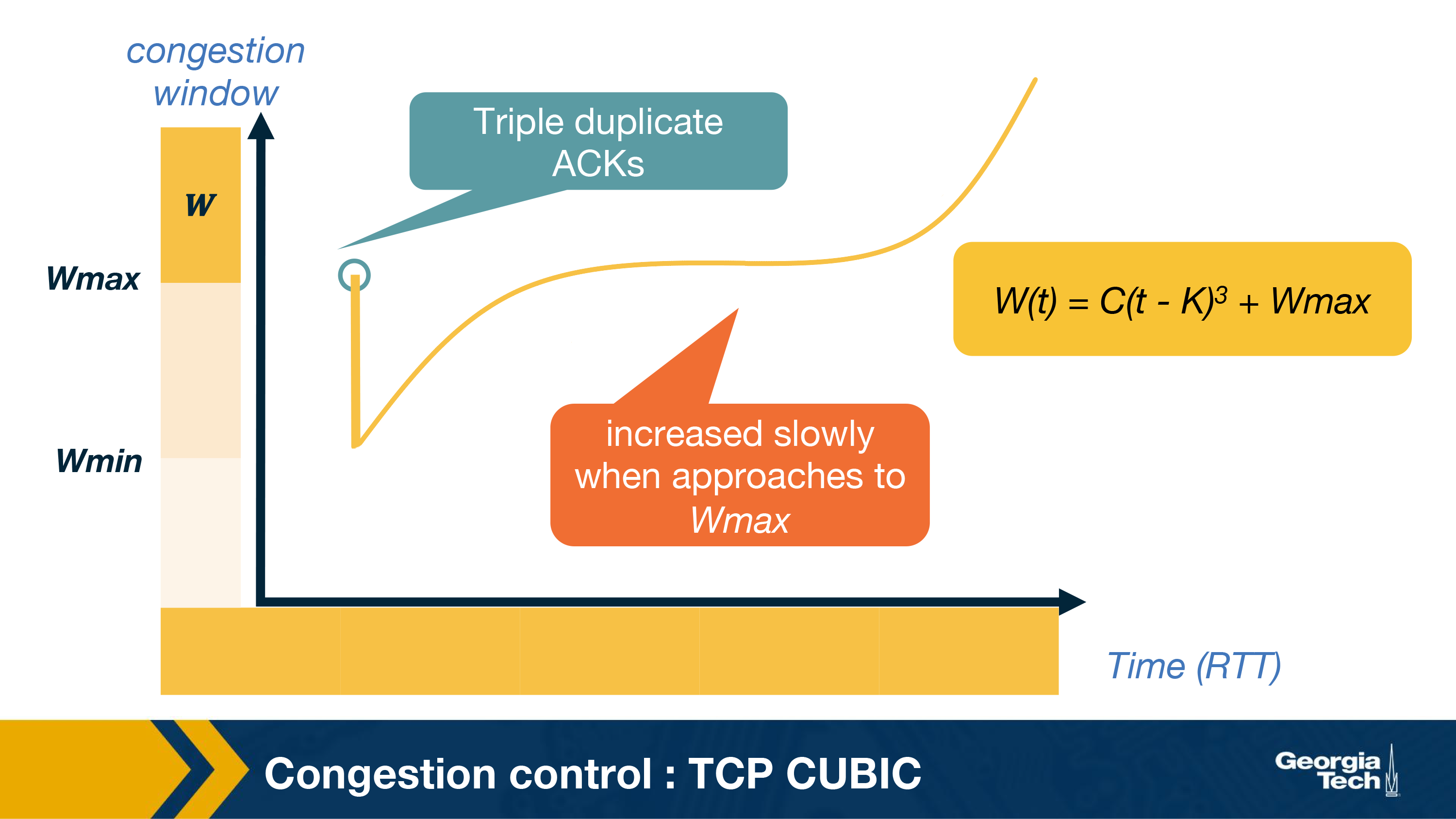
Let us see what happens when TCP experiences a triple duplicate ACK, say at window=Wmax. This could be because of congestion in the network. To maintain TCP-fairness, it uses a multiplicative decrease and reduces the window to half. Let us call this Wmin.
Now, we know that the optimal window size would be in between Wmin and Wmax and closer to Wmax. So, instead of increasing the window size by 1, it is okay to increase the window size aggressively in the beginning. Once the W approaches closer to Wmax, it is wise to increase it slowly because that is where we detected a packet loss last time. Assuming no loss is detected this time around Wmax, we keep on increasing the window a little bit. If there is no loss still, it could be that the previous loss was due to a transient congestion or non-congestion related event. Therefore, it is okay to increase the window size with higher values now.
This window growth idea is approximated in TCP CUBIC using a cubic function. Here is the exact function it uses for the window growth:
W(t) = C(t-K)3 + Wmax
Here, Wmax is the window when the packet loss was detected. Here C is a scaling constant, and K is the time period that the above function takes to increase W to Wmax when there is no further loss event and is calculated by using the following equation:

It is important to note that time here is the time elapsed since the last loss event instead of the usual ACK-based timer used in TCP Reno. This also makes TCP CUBIC RTT-fair.
Explain how in TCP Cubic the congestion window growth becomes independent of RTTs.
The key feature of CUBIC is that its window growth depends only on the time between two consecutive congestion events. One congestion event is the time when TCP undergoes fast recovery. This feature allows CUBIC flows competing in the same bottleneck to have approxi- mately the same window size independent of their RTTs, achieving good RTT-fairness.
The TCP Protocol: TCP Throughput
In a previous topic, we saw that the congestion window follows a sawtooth pattern. As shown in this Figure. The congestion window is increased by 1 packet every RTT, until it reaches the maximum value W, at which point a loss is detected and the cwnd is cut in half, W/2.
Given this behavior, we want to have a simple model that predicts the throughput for a TCP connection.
To make our model more realistic, let's also assume that we have p = the probability loss. So, we assume that the network delivers 1 out of every p consecutive packets followed by a single packet loss.
Because the congestion window (cwnd) size increases a constant rate of 1 packet for every RTT, the height of the sawtooth is W/2 and the width of the base is W/2, which corresponds to W/2 round trips, or RTT * W/2.
The number of packets sent in one cycle the area under the sawtooth. Therefore, the total number of packets sent:
(W/2)2 + 1/2*(W/2)2 = 3/8*W2
As stated in our assumptions about out lossy network, it delivers 1/p packets followed by a loss. So:
1/p = (w/2)2 + 1/2*(w/2)2 = 3/8*W2, solving for W = 
The rate that data that is transmitted is computed as:
BW = data per cycle / time per cycle
Substituting from above:

We can collect all of our constants into  , compute the throughput:

In practice, because of additional parameters, such as small receiver windows, extra bandwidth availability, and TCP timeouts, our constant term C is usually less than 1. This means that bandwidth is bounded by:

Datacenter TCP
At this point, it is important to know that a lot of research has been going in optimizing the congestion control mechanisms. These optimizations are called for because of evolution of the networks. We looked at TCP CUBIC as one such example for high bandwidth delay product networks.
Similarly, data center (DC) networks are other kinds of networks where new TCP congestion control algorithms have been proposed and implemented. There are mainly two differences that have led to this -- the flow characteristics of DC networks are different from the public Internet. There are many short flows that are sensitive to delay. Thus, the congestion control mechanisms are optimized for both delay and throughput and not just the latter alone. Another reason is that DC networks are often owned by a private entity making any changes in the transport layer easier as the new algorithms need not co-exists with the older ones.
DCTCP and TIMELY are two popular examples of TCP designed for DC environments. DCTCP is based on a hybrid approach of using both implicit feedback aka packet loss and explicit feedback from the network using ECN for congestion control. TIMELY uses the gradient of RTT to adjust its window.
OMSCS Notes is made with in NYC by Matt Schlenker.
Copyright © 2019-2023. All rights reserved.
privacy policy