Computer Networks
Router Design and Algorithms (Part 1)
14 minute read
Notice a tyop typo? Please submit an issue or open a PR.
Router Design and Algorithms (Part 1)
What's Inside a Router?
What are the basic components of a router?
The main job of a router is to implement the forwarding plane functions and the control plane functions.
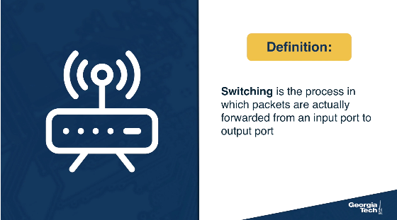
Forwarding (or switching) function:
This is the router's action to transfer a packet from an input link interface to the appropriate output link interface. Forwarding takes place at very short timescales (typically a few nanoseconds), and is typically implemented in hardware.
The router's architecture is shown in the figure below. The main components of a router are the input/output ports, the switching fabric and the routing processor.
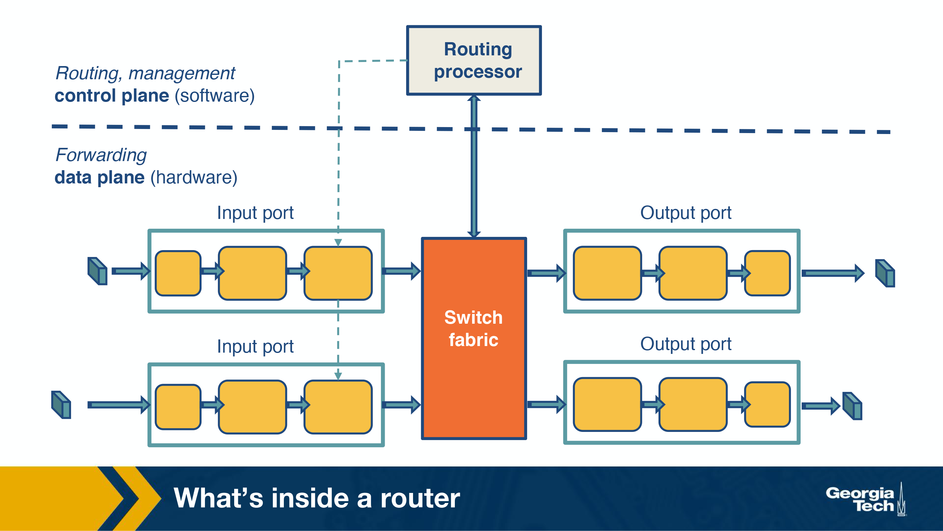
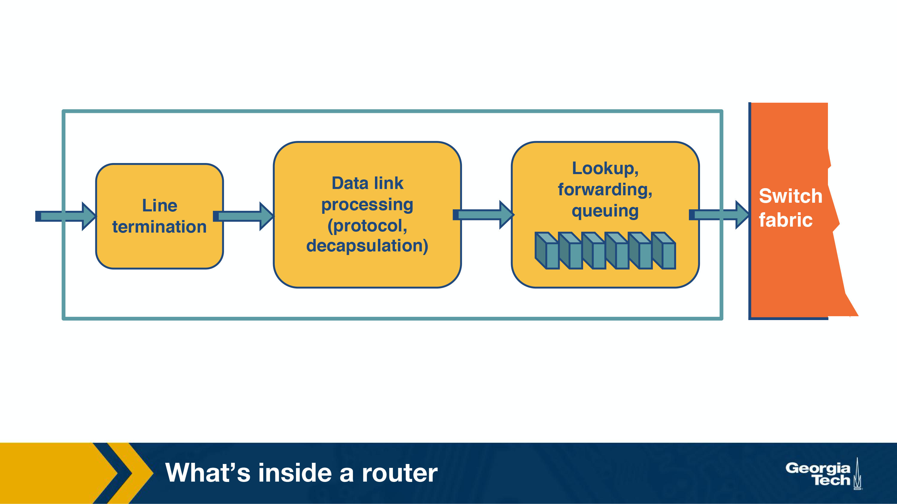
Input ports:
There are several functionalities that are performed by the input ports.
If we look at the figure from left to right, the first function is to physically terminate the incoming links to the router. Second, the data link processing unit decapsulates the packets. Finally, and most importantly, the input ports perform the lookup function. At this point, the input ports consult the forwarding table to ensure that each packet is forwarded to the appropriate output port through the switch fabric.
Switching fabric:
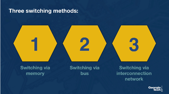
Simply put, the switching fabric moves the packets from input to output ports, and it makes the connections between the input and the output ports. There are three types of switching fabrics: memory, bus, and crossbar.
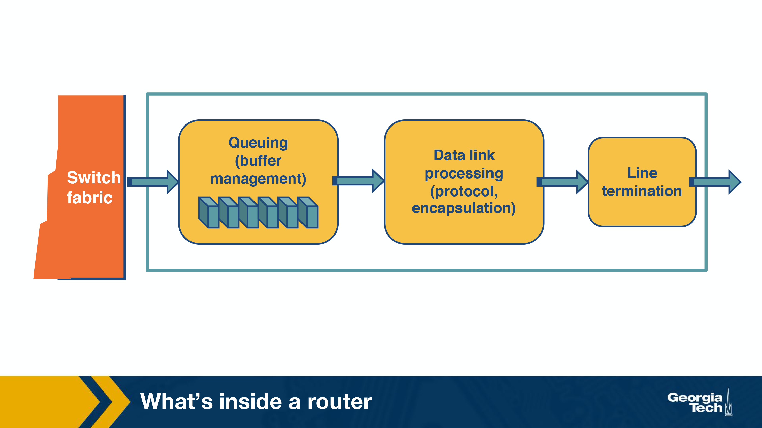
Output ports:
An important function of the output ports is to receive and queue the packets which come from the switching fabric and then send them over to the outgoing link.
Router's control plane functions:
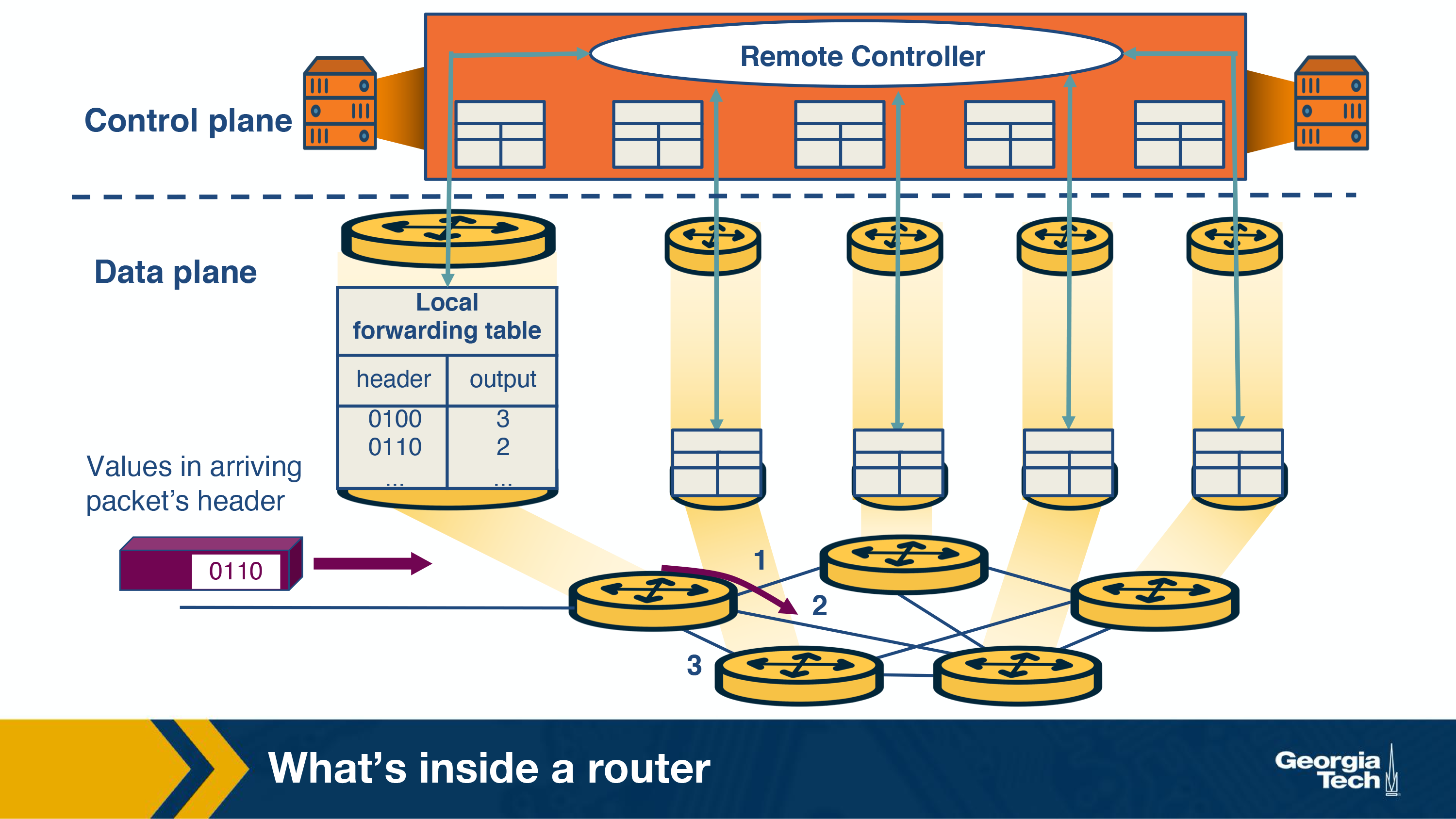
By control plane functions we refer to implementing the routing protocols, maintaining the routing tables, computing the forwarding table. All these functions are implemented in software in the routing processor, or as we will see in the SDN chapter, these functions could be implemented by a remote controller.
Router Architecture
In this topic, we will take a closer look at the router's architecture.
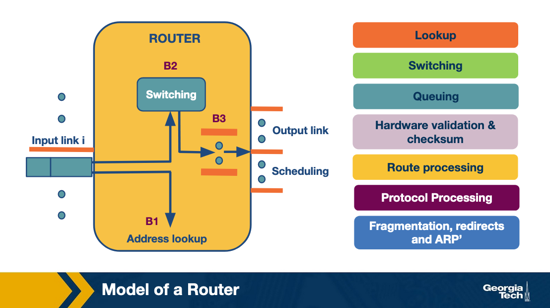
A router has input links and output links and its main task is to switch a packet from an input link to the appropriate output link based on the destination address. We note that in this figure, the input/output links are shown separately but often they are put together.
Now let's look at what happens when a packet arrives at an input link. First, let's take a look at the most time-sensitive tasks: lookup, switching, and scheduling.
Lookup: When a packet arrives at the input link, the router looks at the destination IP address and determines the output link by looking at the forwarding table (or Forwarding Information Base or FIB). The FIB provides a mapping between destination prefixes and output links.
To resolve any disambiguities, the routers use the longest prefix matching algorithms which we will see in a few topics. Also, some routers offer a more specific and complex type of lookup, called packet classification, where the lookup is based on destination or source IP addresses, port, and other criteria.
Switching: After lookup, the switching system takes over to transfer the packet from the input link to the output link. Modern fast routers use crossbar switches for this task. Though scheduling the switch (matching available inputs with outputs) is a difficult task because multiple inputs may want to send packets to the same output.
Queuing: After the packet has been switched to a specific output, it will need to be queue (if the link is congested). The queue maybe as simple as First-In-First-Out (FIFO) or it may be more complex (eg weighted fair queuing) to provide delay guarantees or fair bandwidth allocation.
Now, let's look at some less time-sensitive tasks that take place in the router.
Header validation and checksum: The router checks the packet's version number, it decrements the time-to-live (TTL) field, and also it recalculates the header checksum.
Route processing: The routers build their forwarding tables using routing protocols such as RIP, OSPF, and BGP. These protocols are implemented in the routing processors.
Protocol Processing: The routers, in order to implement their functions, need to implement the following protocols: a) The simple network management protocol (SNMP) that provides a set of counters for remote inspection, b) TCP and UDP for remote communication with the router, c) Internet control message protocol (ICMP), for sending error messages, eg when time to live time is exceeded.
Different Types of Switching
Let's take a closer look into the switching fabric.
The switching fabric is the brains of the router, as it actually performs the main task to switch (or forward) the packets from an input port to an outport port.
Let's look at the ways that this can be accomplished:
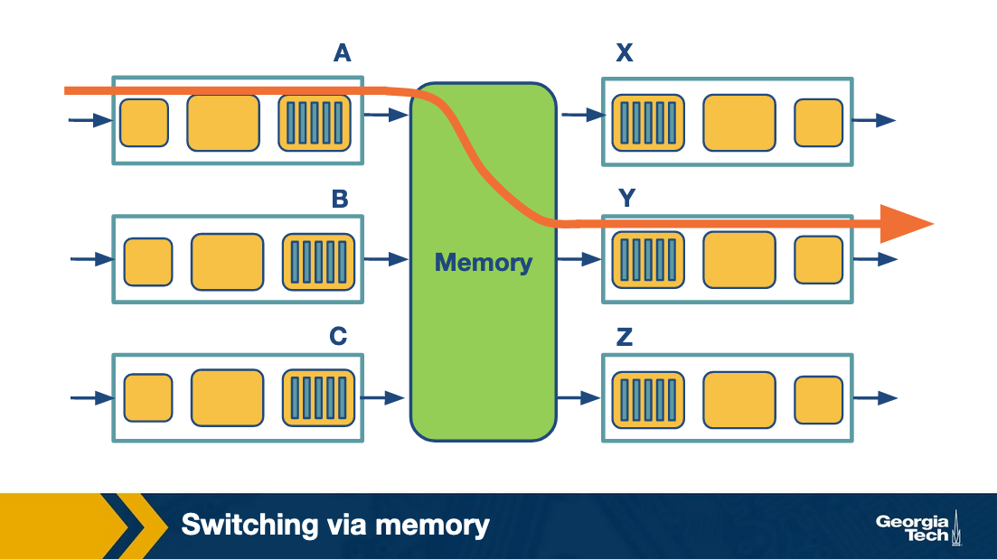
Switching via memory. Input/Output ports operate as I/O devices in an operating system, and they are controlled by the routing processor. When an input port receives a packet, it sends an interrupt to the routing processor and the packet is copied to the processor's memory. Then the processor extracts the destination address and looks into the forward table to find the output port, and finally the packet is copied into that output's port buffer.
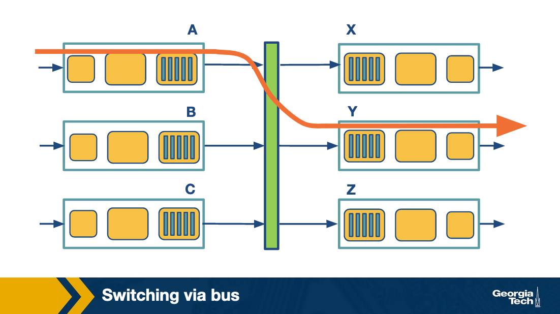
Switching via bus: In this case, the routing processor does not intervene as we saw the switching via memory. When an input port receives a new packet, it puts an internal header that designates the output port, and it sends the packet to the shared bus. Then all the output ports will receive the packet, but only the designated one will keep it. When the packet arrives at the designated output port, then the internal header is removed from the packet. Only one packet can cross the bus at a given time, and so the speed of the bus limits the speed of the router.
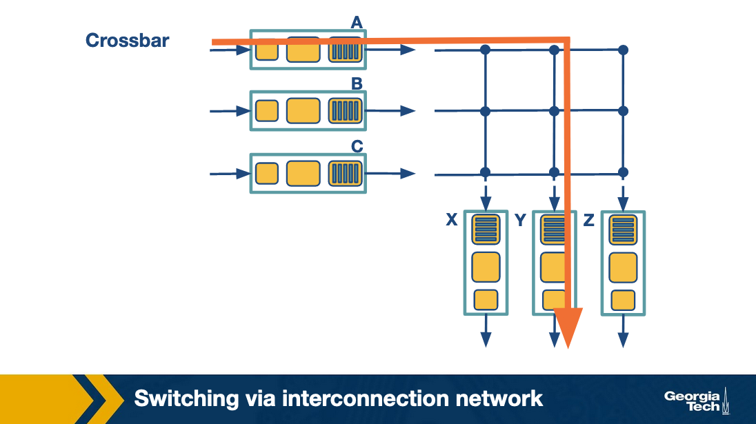
Switching via interconnection network: A crossbar switch is an interconnection network that connects N input ports to N output ports using 2N buses. Horizontal buses meet the vertical buses at crosspoints which are controlled by the switching fabric. For example, let's suppose that a packet arrives at port A that will need to be forwarded to output port Y, the switching fabric closes the crosspoint where the two buses intersect, so that port A can send the packets onto the bus and then the packet can only be picked up by output port Y. Crossbar network can carry multiple packets at the same time, as long as they are using different input and output ports. For example, packets can go from A-to-Y and B-to-X at the same time.
Challenges that the router faces
The fundamental problems that a router faces revolve around:
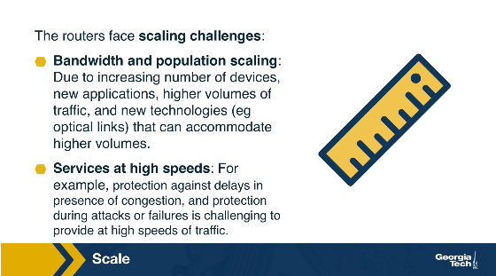
Bandwidth and Internet population scaling: These scaling issues are caused by: a) An increasing number of devices that connect to the Internet, 2) Increasing volumes of network traffic due to new applications, and 3) New technologies such as optical links that can accommodate higher volumes of traffic.
Services at high speeds: New applications require services such as protection against delays in presence of congestion, and protection during attacks or failures. But offering these services at very high speeds is a challenge for routers.
To understand why, let's look at the bottlenecks that routers face in more detail:
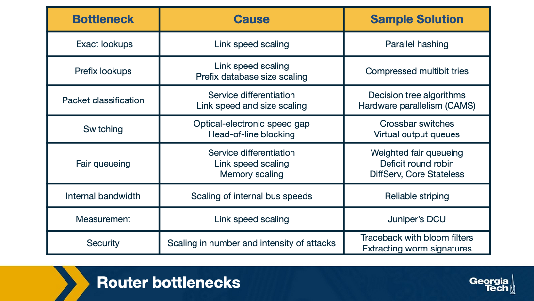
Longest prefix matching. As we have seen in previous topics, routers need to look up a packet's destination address to forward it. The increasing number of the Internet hosts and networks, has made it impossible for routers to have explicit entries for all possible destinations. Instead routers group destinations into prefixes. But then, routers run into the problem of more complex algorithms for efficient longest prefix matching.
Service differentiation. Routers are also able to offer service differentiation which means different quality of service (or security guarantees) to different packets. In turn, this requires the routers to classify packets based on more complex criteria that go beyond destination and they can include source or applications/services that the packet is associated with.
Switching limitations. As we have seen a fundamental operation of routers is to switch packets from input ports to output ports. A way to deal with high-speed traffic, is to use parallelism by using crossbar switching. But in high speeds, this comes with its own problems and limitations (eg head of line blocking).
Bottlenecks about services. Providing performance guarantees (quality of service) in high speeds is nontrivial. Finally, providing support for new services such as measurements and security guarantees.
In the following topics, we explore suggested solutions to deal with these bottlenecks.
Prefix-Match Lookups
What is prefix-match lookup? Why is it required?
In the next topics, we will look into the prefix-matching algorithms. The Internet continues to grow both in terms of networks (AS numbers) and IP addresses. One of the challenges that a router faces is the scalability problem. One way to help with the scalability problem is to “group” multiple IP addresses by the same prefix.
Prefix notation
The different ways to denote prefix are:
-
Dot decimal
Example of 16-bit prefix: 132.234
Binary form of the first octet: 10000100
Binary of second octet: 11101010
Binary prefix of 132.234: 1000010011101010*,
The * indicates wildcard character to say that the remaining bits do not matter.
-
Slash notation
Standard notation: A/L (where A=Address, L=Length)
Example: 132.238.0.0/16
Here, 16 denotes that only the first 16 bits are relevant for prefixing
-
Masking
We can use a mask instead of the prefix length.
Example: The Prefix 123.234.0.0/16 is written as 123.234.0.0 with a mask 255.255.0.0
The mask 255.255.0.0 denotes that only the first 16 bits are important.
What is the need for variable length prefixes?
In the earlier days of the Internet, we used an IP addressing model based on classes (fixed length prefixes). With the rapid exhaustion of IP addresses, in 1993, the Classless Internet Domain Routing (CIDR) came into effect. CIDR essentially assigns IP addresses using arbitrary-length prefixes. CIDR has helped to decrease the router table size but at the same time it introduced us to a new problem: longest-matching-prefix lookup.
Why do we need (better) lookup algorithms?
In order to forward an incoming packet, a router first checks the forwarding table to determine the port and then does switching to actually send the packet. There are various challenges that the router needs to overcome performing a lookup to determine the output port. These challenges revolve around lookup speed, memory, and update time.
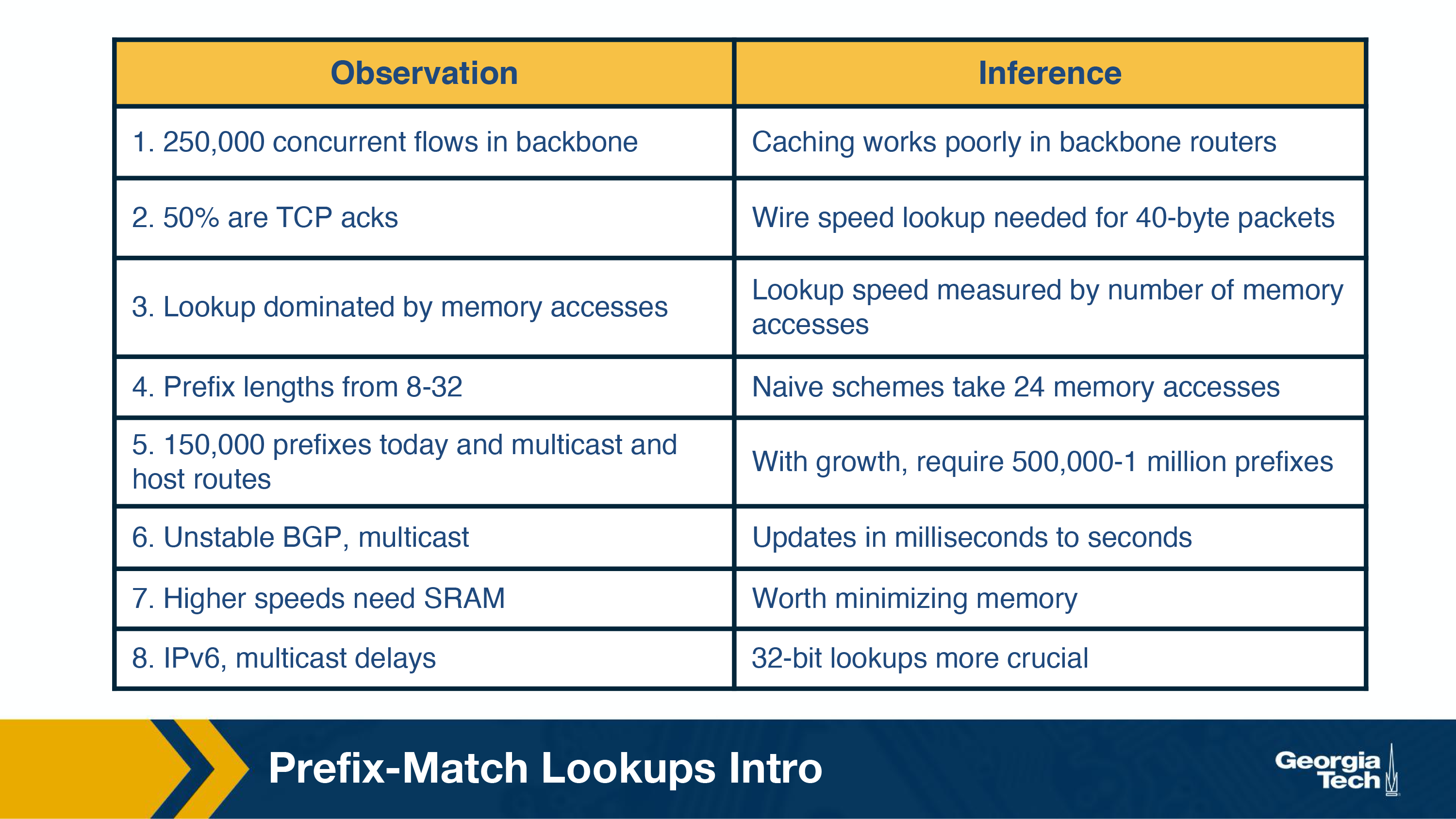
The table below mentions some basic observations around network traffic characteristics. The table shows for every observation, the consequence (inference) that motivates and impacts the design of prefix lookup algorithms. The four take away observations are:
- Measurement studies on network traffic had shown a large number (in the order of hundred thousands, 250,000 according to a measurement study in the earlier days of the Internet) of concurrent flows of short duration. This already large number has only been increasing. This has a consequence that a caching solution would not work efficiently.
- The important element while performing any lookup operation is how fast it is done (lookup speed). A large part of the cost of computation for lookup is accessing memory.
- An unstable routing protocol may adversely impact the update time in the table: add, delete or replace a prefix. Inefficient routing protocols increase this value up to additional milliseconds.
- An important trade-off is memory usage. We have the option to use expensive fast memory (cache in software, SRAM in hardware) or cheaper but slower memory (e.g., DRAM, SDRAM).
Unibit Tries
To start our discussion on prefix matching algorithms, we will use an example prefix database with nine prefixes as shown below.
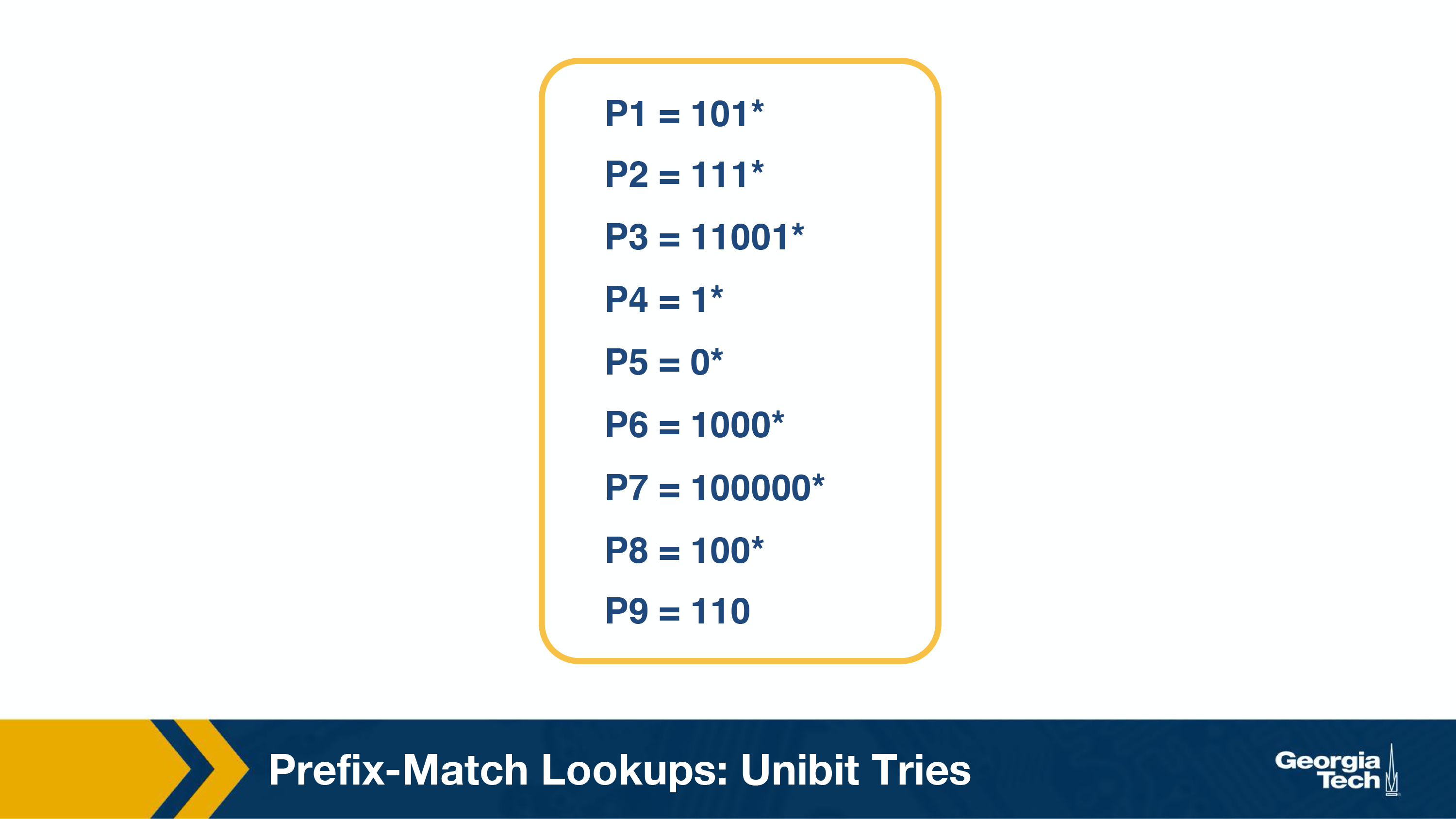
One of the simplest techniques for prefix lookup is the unibit trie. For the example database we have, the figure below shows a unibit trie:
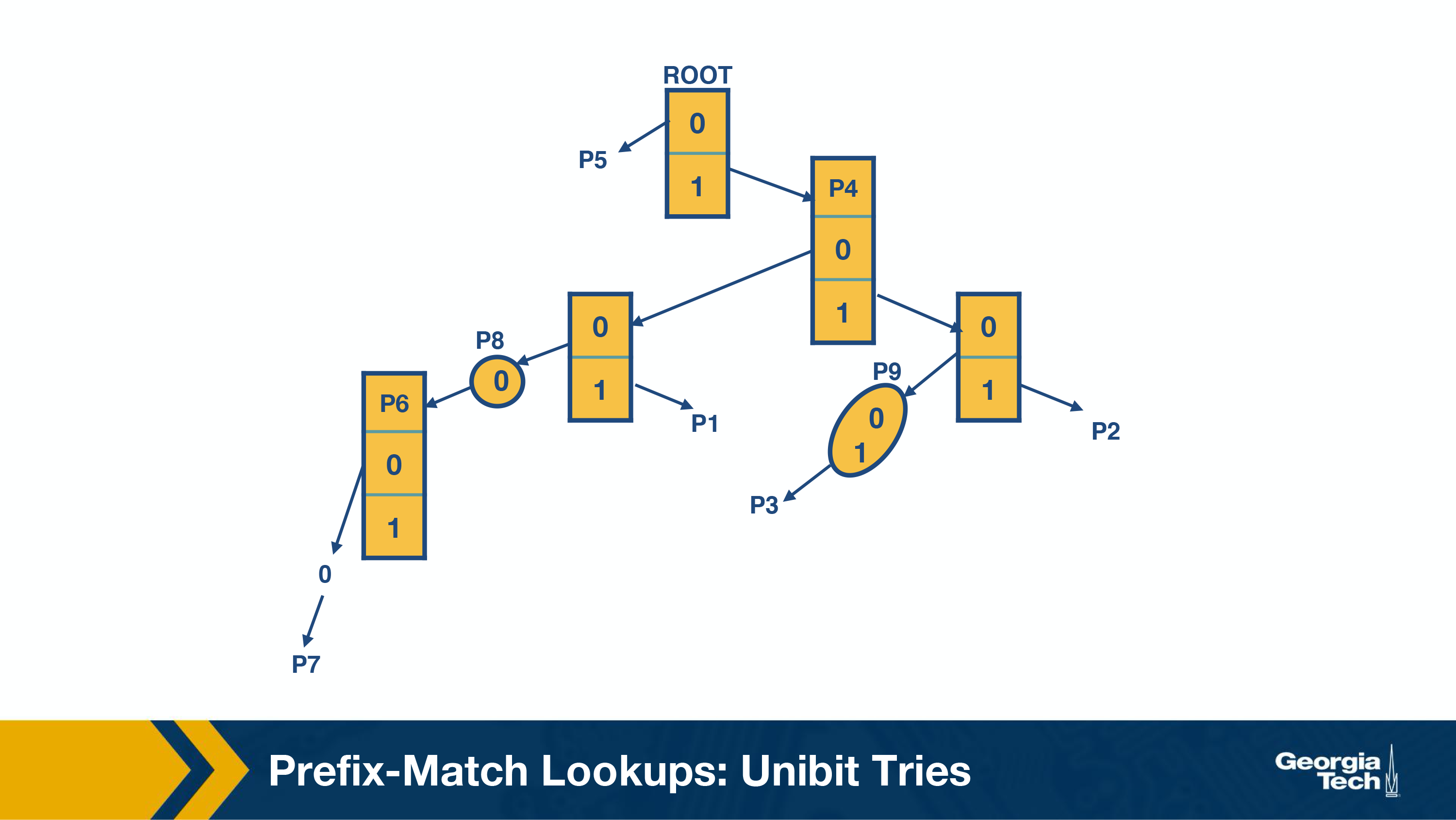
Every node has a 0 or 1 pointer. Starting with the root, pointer 0 points to a subtrie for all prefixes that start with 0, and similarly pointer 1 points to a subtrie for all prefixes that start with 1. Moving forward in a similar manner, we construct more subtries by allocating the remaining bits of the prefix.
When we are doing prefix matching we follow the path from the root node down to the trie. Let's take an example from the above table and see how we can do prefix matching in the unibit trie.
For example:
- Assume that we are doing a longest prefix match for P1=101* (from our prefix database). We start at the root node and trace a 1-pointer to the right, then a 0-pointer to the left and then a 1-pointer to the right
- For P7=100000*, we start at the root node and trace a 1-pointer to the right, then five 0-pointers the left
These are the steps we follow to perform a prefix match:
- We begin the search for a longest prefix match by tracing the trie path.
- We continue the search until we fail (no match or an empty pointer)
- When our search fails, the last known successful prefix traced in the path is our match and our returned value.
Two final notes on the unibit trie:
- If a prefix is a substring of another prefix, the smaller string is stored in the path to the longer (more specific prefix). For example, P4 = 1 is a substring of P2 = 111, and thus P4 is stored inside a node towards the path to P2.
- One-way branches. There may be nodes that only contain one pointer. For example let's consider the prefix P3 = 11001. After we match 110 we will be expecting to match 01. But in our prefix database, we don't have any prefixes that share more than the first 3 bits with P3. So if we had such nodes represented in our trie, we would have nodes with only one pointer. The nodes with only one pointer each are called a one-way branch. For efficiency, we compress these one-way branches to a single text string with 2 bits (shown as node P9).
Multibit Tries
Why do we need multibit tries?
While a unibit trie is very efficient and also offers advantages such as fast lookup and easier updates, its biggest problem is the number of memory accesses that it requires to perform a lookup. For 32 bit addresses, we can see that looking up the address in a unibit trie might require 32 memory accesses, in the worst case. Assuming a 60 nsec latency, the worst case search time is 1.92 microseconds. This could be very inefficient in high speed links.
Instead, we can implement lookups using a stride. By stride we refer to the number of bits that we check at each step.
So an alternative to unibit tries are the multibit tries. A multibit trie is a trie where each node has 2k children, where k is the stride. Next we will see that we can have two flavors of multibit tries: fixed length stride tries and variable length stride tries.
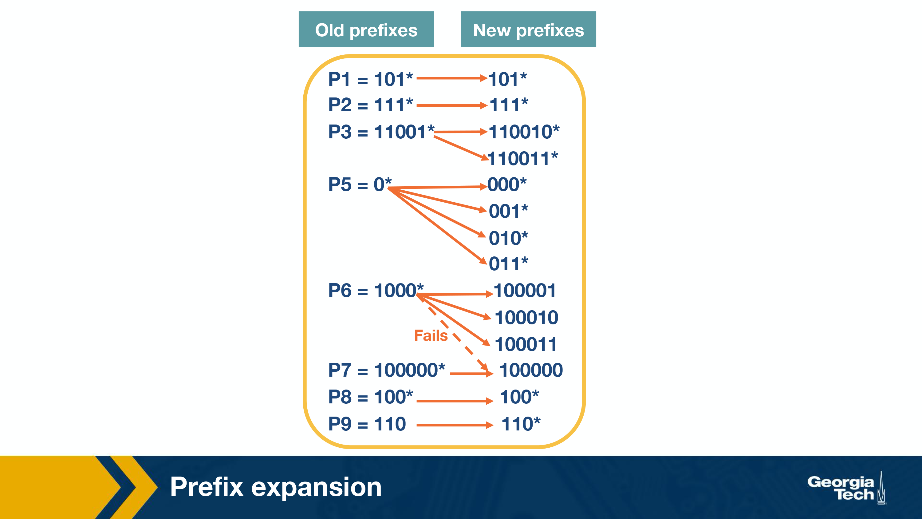
Prefix Expansion
Consider a prefix such as 101 (length 3) and a stride length of 2 bits. If we search in 2 bit lengths, we will miss out on prefixes like 101. To combat this, we use a strategy called controlled prefix expansion, where we expand a given prefix to more prefixes. We ensure that the expanded prefix is a multiple of the chosen stride length. At the same time we remove all lengths that are not multiples of the chosen stride length. We end up with a new database of prefixes, which may be larger (in terms of actual number of prefixes) but with fewer lengths. So, the expansion gives us more speed with an increased cost of the database size.
The figure below shows how we have expanded our original database of prefixes. Originally we had 5 prefix lengths. Now we have more prefixes but only two lengths (3 and 6).
For example we substitute (expand) P3 = 11001 with 110010 and 110011*.
When we expand our prefixes, there may be a collision, i.e. when an expanded prefix collides with an existing prefix. In that case the expanded prefix gets dropped. In the figure, we see that in the fourth expansion of P6=1000* which collides with P7, and thus gets removed.
Multibit tries: Fixed-Stride
As we introduced multibit tries in the previous section, here we will look at a specific example of a fixed-stride trie of length 3. Every node has 3 bits.
We are using the same database of prefixes as in the previous section. We can see that the prefixes (P1, P2, P3, P5, P6, P7, P8 and P9) are all represented in the expanded trie.
Some key points to note here:
- Every element in a trie represents two pieces of information: a pointer and a prefix value.
- The prefix search moves ahead with the preset length in n-bits (3 in this case)
- When the path is traced by a pointer, we remember the last matched prefix (if any).
- Our search ends when an empty pointer is met. At that time, we return the last matched prefix as our final prefix match.
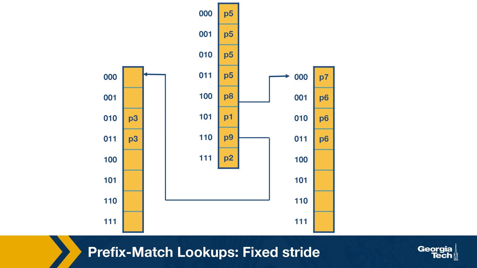
Example: We consider an address A which starts with 001. The search for A starts with the 001 entry at the root node of the trie. Since there is no outgoing pointer, the search terminates here and returns P5. Whereas if we search for 100000, the search would terminate with P7.
Multibit Tries: Variable Stride
Why do we need variable strides?
In this topic, we will talk about a more flexible version of the algorithm which offers us variable number of strides. With this scheme, we can examine a different number of bits every time.
We encode the stride of the trie node using a pointer to the node. The root node stays as is (in the previous scheme).
We note that the rightmost node still needs to examine 3 bits because of P7.
But at the leftmost node need only to examine 2 bits, because P3 has 5 bits in total. So we can rewrite the leftmost node as in the figure below.
So now we have 4 fewer entries than our fixed stride scheme. So by varying the strides we could make the our prefix database smaller, and optimize for memory.
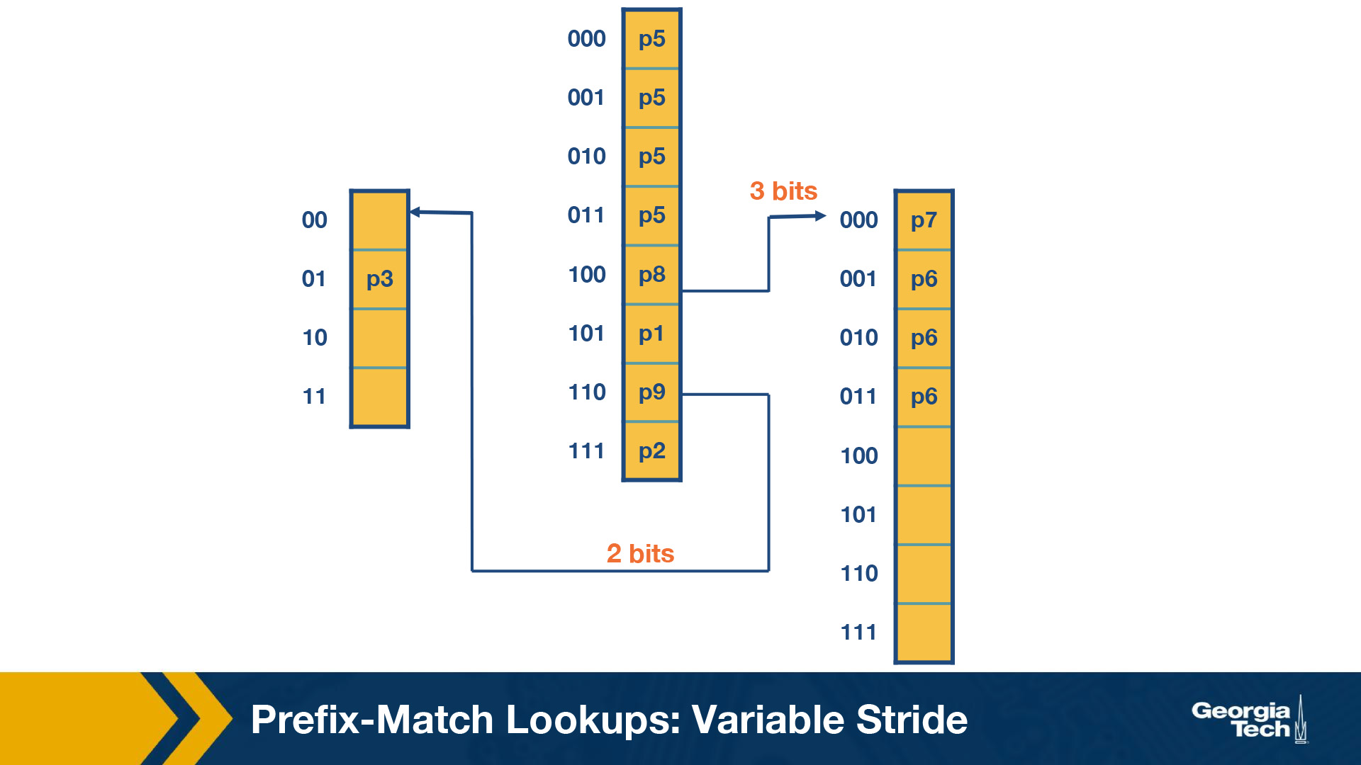
Some key points about variable stride:
- Every node can have a different number of bits to be explored
- The optimizations to the stride length for each node are all done in pursuit of saving trie memory and the least memory access
- An optimum variable stride is selected by using dynamic programming
OMSCS Notes is made with in NYC by Matt Schlenker.
Copyright © 2019-2023. All rights reserved.
privacy policy