Computer Networks Old
Switching
10 minute read
Notice a tyop typo? Please submit an issue or open a PR.
Switching
Switching and Bridging
In this lesson, we will learn about how hosts find each other on a subnet and how subnets are interconnected.
We will also learn about the difference between switches and hubs, and switches and routers.
We will also talk about the scaling problems with ethernet and mechanisms we can use to allow it scale better.
Bootstrapping: Networking Two Hosts
A host that wants to send a datagram to another host can simply send that datagram via its ethernet adapter with a destination MAC address of the host that it wants to receive the frame.
Frames can also be sent to a broadcast destination MAC address which would mean that the datagram would be sent to every host it was connected to on the local area network.
Typically, a host knows a DNS name or IP address of another host, but it may not know the hardware/MAC address of the adapter on the host that it wants to communicate with.
We need to provide a way for a host to learn the MAC address of another host. We can do this via the Address Resolution Protocol (ARP).
ARP: Address Resolution Protocol
In ARP, a host queries with an IP address, broadcasting that query to every other node on the network. The host that has the IP address on the LAN will respond with the appropriate MAC address.
The ARP query is a broadcast that goes to every host on the LAN, and the response is a unicast with the MAC address to the host that issued the query.
When the host that issued the reply receives a response, it begins to build an ARP table, which maps IP address to MAC addresses.
In the future, the host will consult the ARP table to get the MAC address for a given IP address instead of issuing an ARP query out into the network.
When the host wants to send a packet to a destination with a particular IP address, it takes the IP packet and encapsulates it in an ethernet frame with the corresponding destination MAC address.
Interconnecting LANs with Hubs
The simplest way that a LAN can be connected is with a hub. A hub essentially creates a broadcast medium among all of the connected hosts, where all packets on the network are seen everywhere.
If a particular host sends a frame that is destined for another host on the LAN, the hub will broadcast that frame out every outgoing port, so all packets will be seen everywhere.
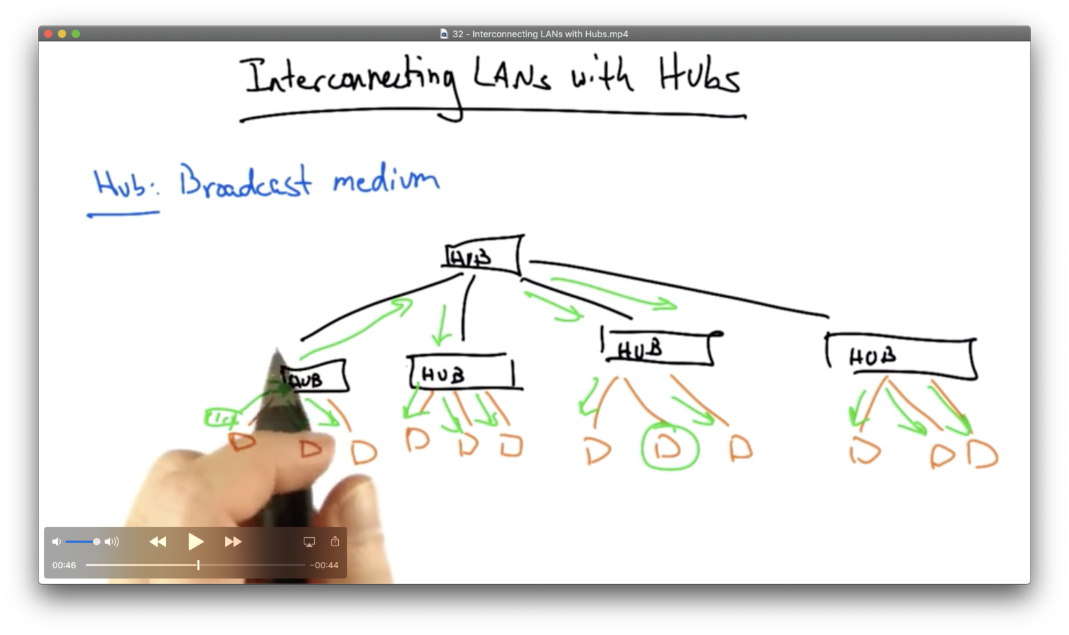
There is a lot of flooding and there are many chances for collision. The chance of collision introduces additional latency in the network, because collision requires other hosts to back off and not send as soon as they see other senders trying to send at the same time.
LANs that are connected with hubs are also vulnerable to failures or misconfigurations. Even one misconfigured device can cause problems for every other device on the LAN.
We need to improve on this broadcast medium by imposing some amount of isolation.
Switches: Traffic Isolation
In contrast, switches provide some amount of traffic isolation so that the entire LAN doesn't become one broadcast medium.
A switch will partition the LAN into separate broadcast/collision domains, or segments. A frame that is bound for a host in the same LAN segment will only be broadcast within that segment. The switch will not broadcast it to other segments.
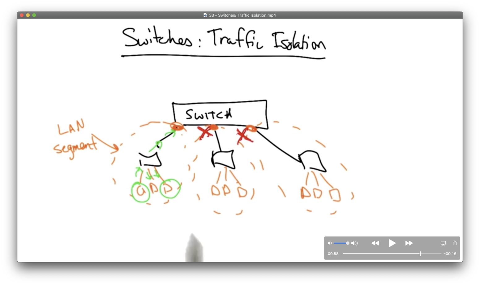
Enforcing this type of isolation requires constructing a switch table at the switch which maps destination MAC addresses to switch output ports.
Learning Switches
A learning switch maintains a table that maps destination addresses to output ports on the switch.
When a learning switch receives a frame destined for a particular address, it knows what output port to forward the frame.
Initially, the forwarding table is empty. If there is not an entry in the forwarding table for a given destination address, the switch will just flood all of its output ports.
For example, consider a switch that is receiving a frame from A, destined for C, on port 1. If the switch has no entry for C, the switch will flood. Note that the switch will be able to create an entry mapping destination A to port 1, since the frame with a source of A arrived at port 1.
Learning switches do not completely eliminate flooding. They have to flood in the case when destination/port mapping are not present, and they must also flood in the case of broadcast frames, like ARP.
Most underlying physical topologies have loops for reasons of redundancy. If a given link on the LAN fails, we still wants hosts to be connected.
When two switches are connected in a loop, and one sends a broadcast frame, the other switch will receive it, and broadcast it back out. The first switch will receive it again and rebroadcast it again. This is often referred to as a forwarding loop or broadcast storm.
We need a solution to ensure that the switches don't always flood all packets on all outgoing ports. We need a protocol to create a logical forwarding tree on top of the underlying physical topology.
Spanning Tree
A spanning tree is a loop-free topology that covers every node in a graph.
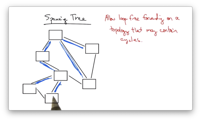
Instead of flooding a frame, a switch in this topology would simply forward packets along the spanning tree, not across all output links.
In order to construct a spanning tree, a collection of nodes must first elect a root - every tree must have a root. Typically, the switch with the smallest ID is the root.
Each switch must then decide which of its links to include in the spanning tree. The switch will exclude any link that is determined not on the shortest path to the root.
For example, suppose a switch has three outgoing links: A, B, and C. The root can be reached via link A in three hops, via link B in two hops, and via link C in one hop. The switch will include link C in its spanning tree.
How do we determine the root in the first place?
Initially, every node thinks that it is the root, and the switches run an election process to determine which switch has the smallest ID. If a switch learns of a switch with a smaller ID, it updates its view of the root and computes its distance from the new root.
Whenever a switch updates its view of the root, it also determines how far it is from the root so that when other neighboring nodes receive updates they can determine their distance to new root simply by adding one to any message that they receive.
Spanning Tree Example
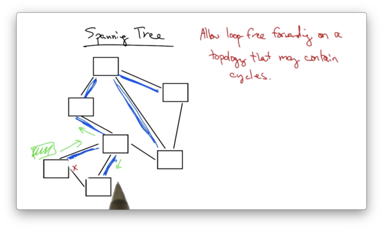
Assume that nodes message each other using the format (Y, d, X) where X is the originating node, d is the distance from X to the current claimed root, and Y is the current claimed root.
Initially, every node thinks that it is the root, so every node will broadcast (X, 0, X) .
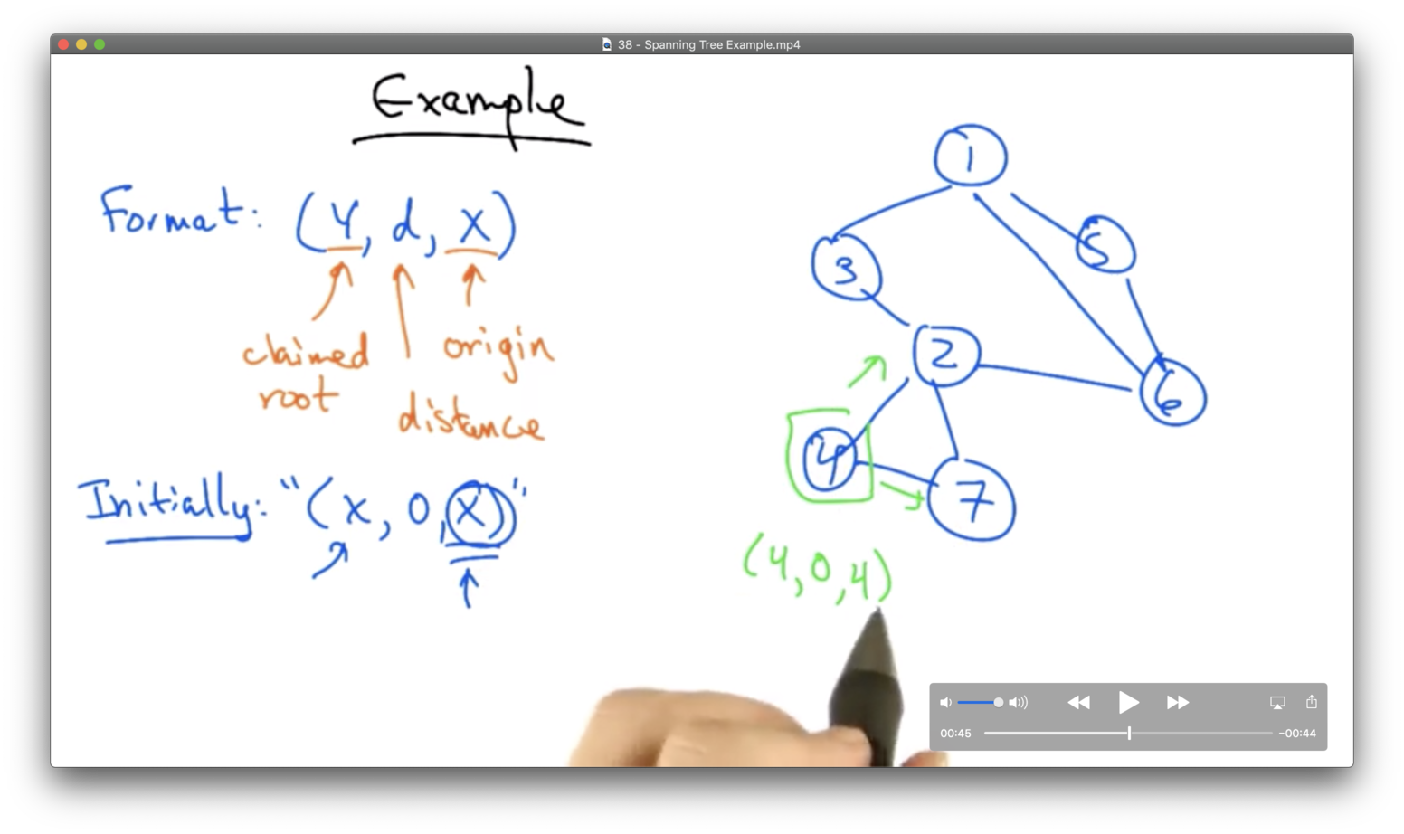
Consider node 4 above.
Initially, node 4 sends out (4, 0, 4) to node 7 and node 2. Node 4 will also receive (2, 0, 2) from node 2. Node 4 will update its view of the root to be node 2. Eventually, node 4 will also hear (2, 1, 7) from node 7, indicating that node 7 thinks that it is one hop away from the root.
Node 4 will then realize that the path through node 7 is a longer path than the path directly to node 2, and it will drop the link to node 7 from its spanning tree.
Switches Vs Routers
Switches typically operate at layer two (the link layer). A common layer two protocol is Ethernet.
Switches are typically auto-configuring, and forwarding tends to be quite fast, since packets processing in layer two consists only of flat lookups.
Routers typically operate at layer three - the network layer - where IP reigns. Router level topologies are not restricted to spanning trees. For example, in multi path routing, a single packet can be sent along one of several possible paths in the underlying router-level topology.
Layer two switching is a lot more convenient, but a major limitation is broadcast. The spanning tree protocol messages and ARP queries both impose a fairly high load on the network.
Is it possible to get the benefits of layer two switching - auto-configuration and fast forwarding - without the broadcast limitations?
Buffer Sizing
While it is well known that switches and routers do need packet buffers to accommodate for statistical multiplexing, it is less clear how much buffering is actually necessary.
Let's suppose that we have a path between a source and a destination that includes one router.
Assume that the round trip (propagation delay) is 2T (measured in seconds), and the capacity of the bottleneck link is C, (measured in bits/seconds). The commonly held view is that this router need a buffer of size 2T * C (with units of bits).
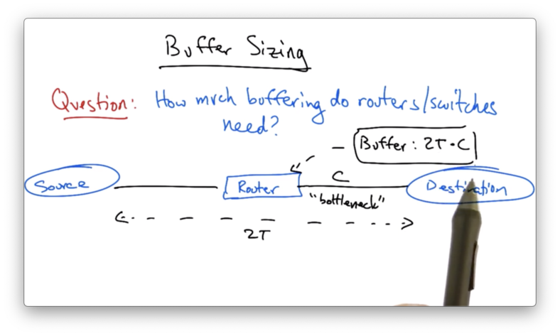
The quantity 2T * C essentially refers to the number of bits that could be outstanding on this path at any given time.
This rule of thumb was mandated in many backbone and edge routers for many years, and appears in RFCs and IETF guidelines. It has major consequences for router design, because these buffers can occupy a lot of router memory, which can get expensive.
In addition, the bigger the buffers, the bigger the queuing delay. This means that interactive traffic may experience larger delays, and hosts may experience larger delays with regard to feedback about congestion in the network.
Buffer Sizing for a TCP Sender
Suppose that we have a TCP sender that is sending packets, where the sending rate is controlled by the congestion window cwnd, and the sender is receiving ACKs.
With a window cwnd, only cwnd unacknowledged packets may be in flight at any time. The source's sending rate R , then, is simply the window cwnd, divided by the round-trip time, RTT.
Remember that TCP uses an additive increase, multiplicative decrease (AIMD) strategy for congestion control.
For every cwnd ACKs received, we send cwnd + 1 packets, up to the the receiver window, rwnd.
We start sending packets using some window cwnd_max / 2 and increase this window additively up to cwnd_max. When we see a drop, we apply multiplicative decrease, and reduce our window - and thus our sending rate - back to cwnd_max / 2 again.
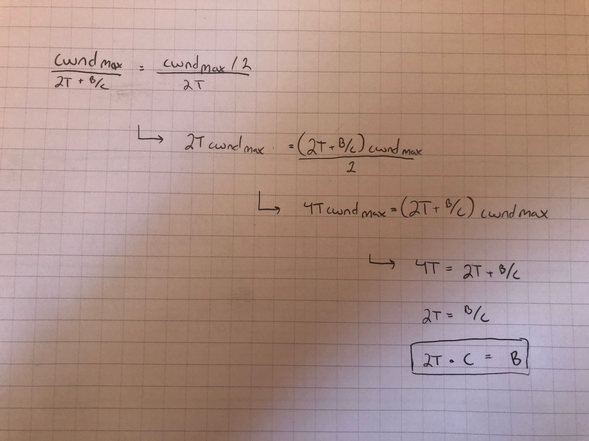
We'd like the sender to send a common rate R before and after the packet drop. Thus:
cwnd_max / RTT_old = (cwnd_max / 2) / RTT_new
The round-trip time is controlled by two factors: the propagation delay, and the queueing delay. The propagation delay is 2T, while the queueing delay is B/C, where B is the size of the buffer at the bottleneck link and C is the transmission rate of the bottleneck link.
We have both propagation delay and queueing delay before the drop.
When the drop occurs, the router buffer contains cwnd_max packets. The sender drops its window size to cwnd_max / 2 and then waits for cwnd_max / 2 ACKs before sending more packets.
The delay from router to destination (for packet transmission) is the same as the delay from destination back to router (for ACK transmission). A second packet can be in flight from router to destination while the ACK of the first packet is in flight from destination back to router. For every ACK that has been received by the sender, two packets have left the router and have been processed by the sender. By the time cwnd_max / 2 ACKs have been received, cwnd_max packets have left the router buffer. The router buffer will be empty.
All this to say: we only have propagation delay - not queueing delay - after the drop. The queue is empty by the time we start retransmitting packets
As a result, RTT_old = 2T + (B/C) and RTT_new = 2T. Thus:
The rule of thumb makes sense for a single flow, but a router in a typical backbone network has more than 20,000 flows.
It turns out that this rule of thumb only really holds if all of those 20,000 flows are perfectly synchronized. If the flows are desynchronized, it turns out that the router can get away with a lot less buffering.
If TCP Flows are Synchronized
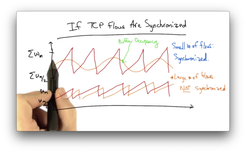
If the TCP flows are synchronized, then the dynamics of aggregate window will have the same characteristics as any individual flow.
If there are only a small number of flows in the network, these flows may tend to stay synchronized, and the aggregate dynamics may mimic the dynamics of any single flow.
As the network begins to support an increasingly larger number of flows, the individual TCP flows become desynchronized.
Individual flows may see peaks at different times. Instead of seeing a large sawtooth - which would be the sum of a number of synchronized flows - the aggregate window will look much smoother.
We can represent the buffer occupancy as a random variable which will, at any given time, take on a range of values, which can be analyzed by the central limit theorem.
The central limit theorem tells us that the more variables (unique congestion windows of TCP flows) we have, the narrower the Gaussian will be. In this case, the Gaussian is the fluctuation of the sum of all of the congestion windows.
The width of the Gaussian decreases as 1/sqrt(n) where n is the number of unique congestion windows.
As a result, the required buffering for a router handling a large number of flows drops from 2T * C to (2T * C) / sqrt(n).
OMSCS Notes is made with in NYC by Matt Schlenker.
Copyright © 2019-2023. All rights reserved.
privacy policy