Computer Networks Old
Naming, Addressing & Forwarding
17 minute read
Notice a tyop typo? Please submit an issue or open a PR.
Naming, Addressing & Forwarding
IP Addressing
In this lesson, we will be covering IPv4 address structure and allocation.
Each IP address is a 32-bit number which is formatted in dotted-quad notation. For example, the IP address for cc.gatech.edu is 130.207.7.36.
130.207.7.36 is just a convenient (base 10) way to write a 32-bit number.
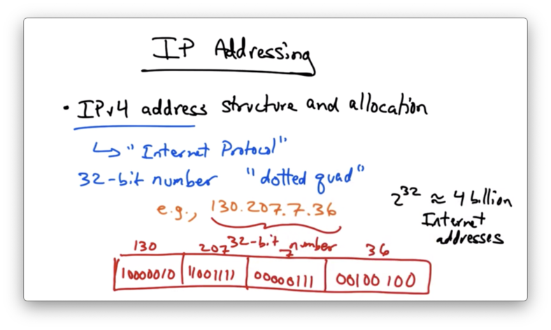
This address structure allows for 2^32 - roughly 4 billion - Internet addresses. While this sounds like a lot of addresses, we are actually running out of IP addresses.
Imagine storing every single IP address in a table. Very quickly, that becomes an extremely large table, where lookups can be slow and the amount of required memory may be very expensive.
We need a concise way of grouping IP addresses.
Pre-1994: "Classful" Addressing
Before 1994, addresses were divided into a network ID portion and a host ID portion.
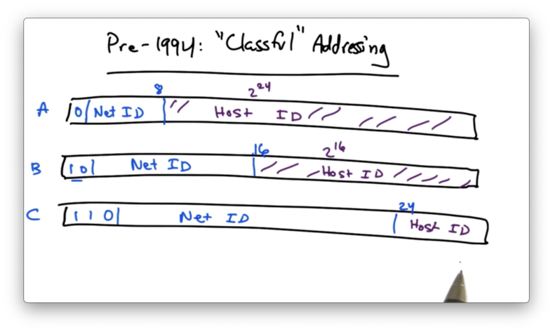
For class A addresses, the first bit is 0. The next 7 bits represent the network ID - the network that owns this portion of the address space. The remaining 24 bits are dedicated for hosts on this network. This means that there are 2^7 class A networks, which can each support 2^24 hosts.
For class B addresses, the first two bits are 10. The next 14 bits signified the network ID, and the remaining 16 bits specified the host ID. This means that there are 2^14 class B networks, which can each support 2^16 hosts.
For class C addresses, the first three bits are 110. The next 21 bits comprise the network ID, while the remaining 8 bits are designated for the host ID. This means that there are 2^21 class C networks, which each can support 2^8 hosts.
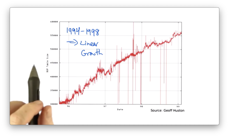
If we look at the size of the BGP routing table, as a function of the year, we can see that the routing table size grew from 1989 to 1994.
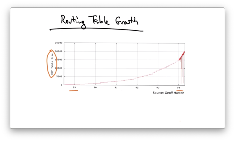
Around 1994, the growth rate of the BGP routing tables began to accelerate, and the rates began to exceed the advances in hardware and software capabilities.
There was another problem as well. There were far more networks that needed just a handful of IP addresses - what class C offered. However, since there was a fixed range for this address space, we began to run out of class C addresses quickly.
We needed more flexible IP address allocation. The solution is classless interdomain routing, or CIDR.
IP Address Allocation
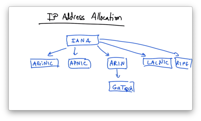
At the top of IP address allocation hierarchy is an organization called the Internet Assigned Numbers Authority (IANA)
IANA has the authority to allocate address space to regional routing registries
- AfriNIC for Africa
- APNIC for Asia and Australia
- ARIN for North America
- LACNIC for Latin America
- RIPE for Europe
Regional routing registries in turn allocate address space to individual networks, like GATech.
The address space allocation across regional routing registries is far from even.
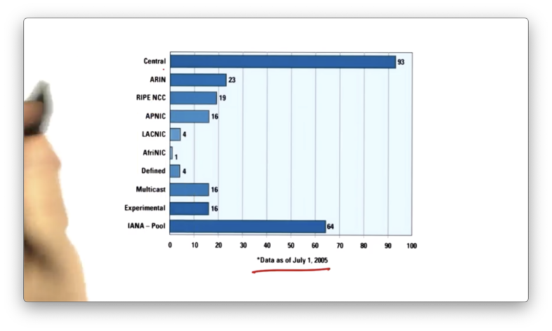
This chart shows the number of /8 address allocations that have been allocated to each of the registries. As of 2005, North America has 23 /8 addresses but the entire continent of Africa only has 1!
Recently, IANA has allocated the remaining /8 address blocks, meaning that we are essentially out of IPv4 addresses.
Querying an IP address using whois and a routing registry - such as ra.net - will give you ownership info about that particular prefix.
For example, querying the IP address 130.207.7.36 tells us that this IP address comes from a /16 allocation, that Georgia Tech is the owner of the prefix, and the IP address is associated with autonomous system AS2637.
Classless Interdomain Routing
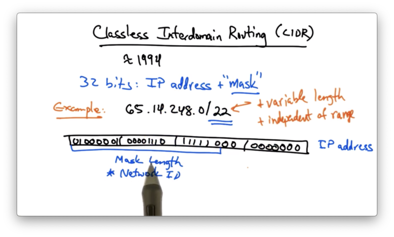
The pressure on address space usage spurred the adoption of classless interdomain routing (CIDR) .
Instead of having fixed network ID and host ID portions of the 32 bits, with CIDR, we would simply have the IP address and a mask. The mask would be of variable length and would indicate the length of the network ID.
For example, consider the IP address 65.14.248.0/22. In this case, the /22 says that the first 22 bits should represent the network ID, which means that the remaining 10 bits represent the host.
This allows those allocating IP address ranges to both allocate a range that is more fitting to the size of the network and also not have to be constrained about how big the network ID should be depending on where in the address space the prefix is being allocated from.
One complication is that we can now have overlapping address prefixes. For example, 65.14.248.0/24 overlaps with 65.14.248.0/22 . The /24 address is actually a subnet of the /22.
What should we do if both of these entries show up in an internet routing table? The solution is to forward on the longest prefix match. Intuitively this makes sense: the prefix with the longer mask length is more specific than the prefix with the shorter mask.
Longest Prefix Match
Every packet has a destination IP address. At each hop, a router looks up the a table entry that matches the destination address to determine where to forward the packet.
This forwarding table will have a number of prefixes in it, and many of those prefixes may be overlapping.

When we see an IP address that may match on the one or more prefixes in this table, we simply match that IP address to the entry in the forwarding table with the longest matching prefix.
One benefit of CIDR and longest prefix matching is efficiency, since prefix blocks can be allocated on a much finer granularity than with classful interdomain routing.
Another benefit of longest prefix matching is aggregation, whereby an upstream network may condense the prefixes advertised to it by downstream network into a shorter prefix to advertise to the rest of the internet.
For example, consider two networks A and B, which each have /16 blocks allocated to them. If all traffic flows to them from the same upstream network C, C may condense the the two /16 blocks into one /8 prefix that it advertises to the rest of the internet. This allows for routers upstream of C to maintain only one /8 entry in their forwarding tables instead of two /16 entries.
CIDR had a significant effect on slowing the growth of the internet routing tables from 1994 to 1998.
Around 2000, fast growth in routing tables resumed.
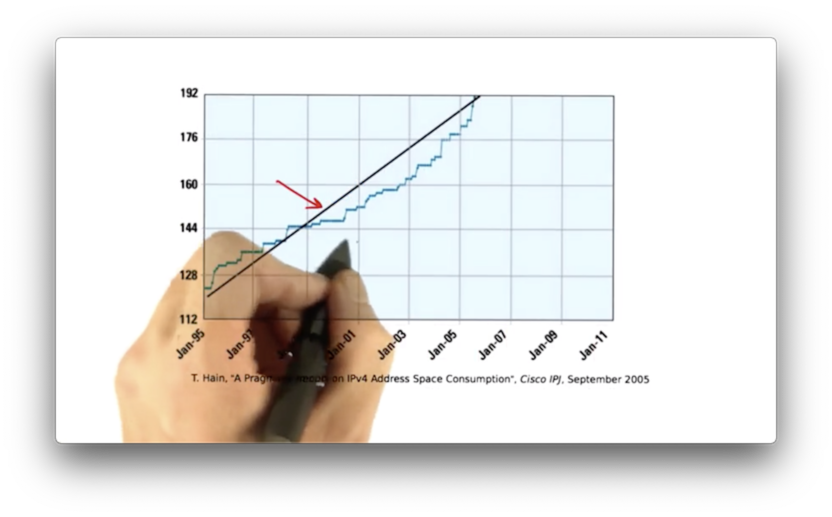
A significant contributor to this growth was a practice called multihoming. Multihoming can make it difficult for upstream providers to aggregate prefixes together, often requiring an upstream provider to store multiple IP prefixes for a single autonomous system.
Multihoming Frustrates Aggregation
Let's consider that following example.
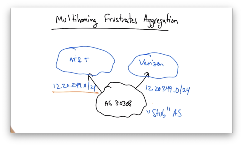
AS 30308 might receive an allocation - say 12.20.249.0/24 from one of its providers. Let's suppose that it receives this allocation from AT&T, which owns 12.0.0.0/8.
Let's suppose that AS 30308 wants to be reachable both by AT&T and Verizon. That is, AS 30308 wants to be multi-homed. To do this, AS 30308 needs to advertise its prefix via both AT&T and Verizon.
The problem occurs when AT&T and Verizon want to advertise that prefix to the rest of the Internet.
AT&T can't aggregate this /24 prefix into 12.0.0.0/8, because then Verizon would be advertising the longer 12.20.249.0/24. This would mean that all traffic for AS 30308 would be routed through Verizon.
As a result, AT&T and Verizon must both advertise the /24 to the rest of the Internet.
The desire to multi-home by small ASes with masks led to an explosion of /24 entries in the global routing table, with many missed opportunities for aggregation that would have otherwise been present.
Longest Prefix Match to Control Inbound Traffic
Suppose AS A owns 10.1.0.0/16 and it advertises its prefix out to both of its upstream links, which advertise them out further.
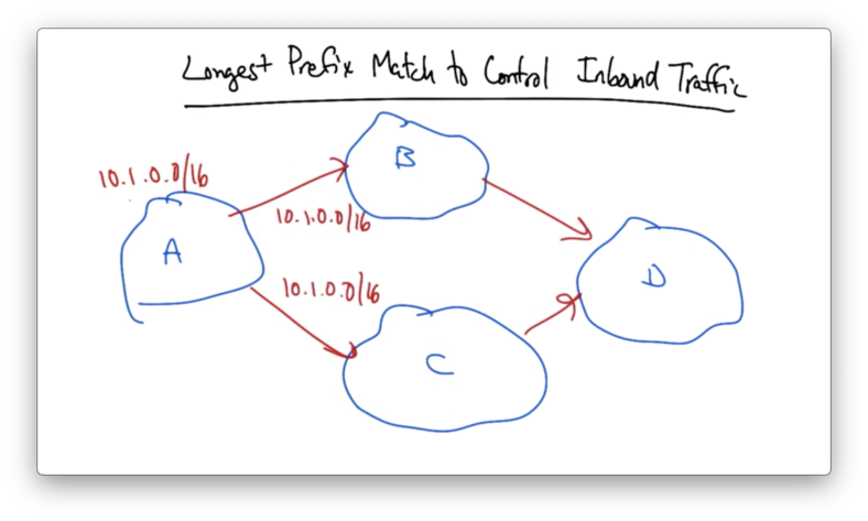
Given an advertisement of one prefix upstream, AS D is going to pick one best BGP route by which to send traffic back to A.
Let's suppose that A, wanted to balance its traffic across its incoming links. A could essentially split its /16 in half, advertising one /17 to B and the other /17 to C.
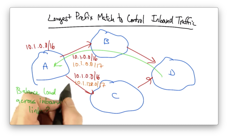
If either link fails, the shorter /16 will ensure that the prefix remains reachable through the other link.
While load balancing is a perfectly good reason for an AS to de-aggregate its prefixes, de-aggregation is often done unnecessarily.
The CIDR report, released weekly, shows top offending ASes who are advertising IP prefixes that are contiguous and could be aggregated.
The report shows basically shows how many unique prefixes an AS is advertising as well as how many unique prefixes could be advertised with maximum aggregation.
The CIDR report might be overly optimistic, as we have just seen that fine reasons for de-aggregation do exist.
Nonetheless, the report shows that there are probably many more IP prefixes in the global internet routing table than there could be if ASes took full advantage of aggregation.
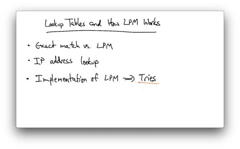
Lookup Tables and How LPM Works
Lookup Algorithm Depends on Protocol
The lookup algorithm that a router uses depends on the protocol that it's using to forward packets.
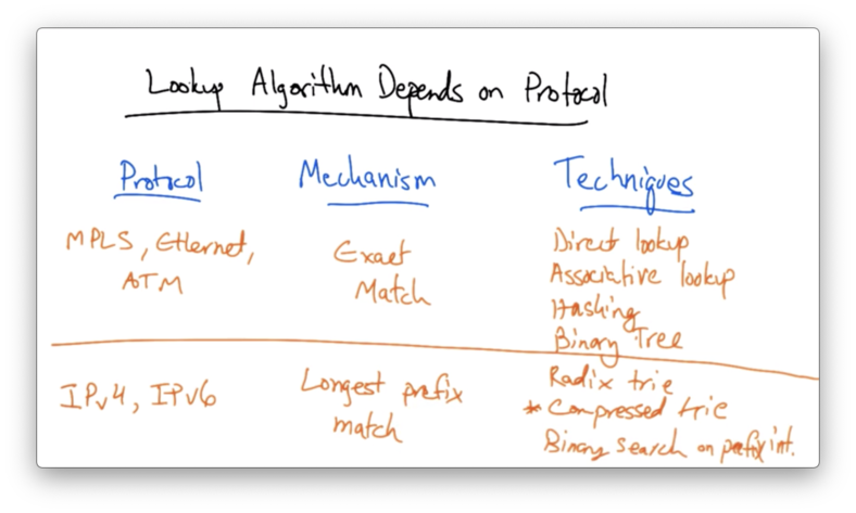
Ethernet
Ethernet forwarding is based on an exact match of a layer 2 address, which is usually 48 bits long. The address is global and the size of the address is not negotiable. It is not possible to hold 2^48 addresses in a table and use direct lookup.
The advantages of exact matches in Ethernet switches is that exact match is simple, and the expected lookup time is O(1). The disadvantages include inefficient use of memory, which potentially results in non-deterministic look up time if a lookup requires multiple memory accesses.
IP Lookups Find Long Prefixes
Suppose that we want to represent an IP address as one point in the space from 0 to 2^32-1 - the range of all 32-bit IP addresses.
Each prefix represents a smaller range inside the larger range of 32 bit numbers and, of course, these ranges may be overlapping.
The idea with longest prefix match is to find the prefix covering the smallest range of IP addresses which includes the specified IP address.
The smaller the range, the larger the prefix.
LPM is harder to perform than exact match! Since the destination IP does not indicate the length of the longest matching prefix, some algorithm must determine it.
We need a way to search all prefix lengths as well as prefixes of a given length.
LPM in IPv4 Exact Match
Suppose we wanted to implement longest prefix match for IPv4 using exact match.
In this case, we might take our IP address and send it to a bunch of different exact match tables. Among the tables that had a match, we would select the longest, and forward the packet out the appropriate output port.
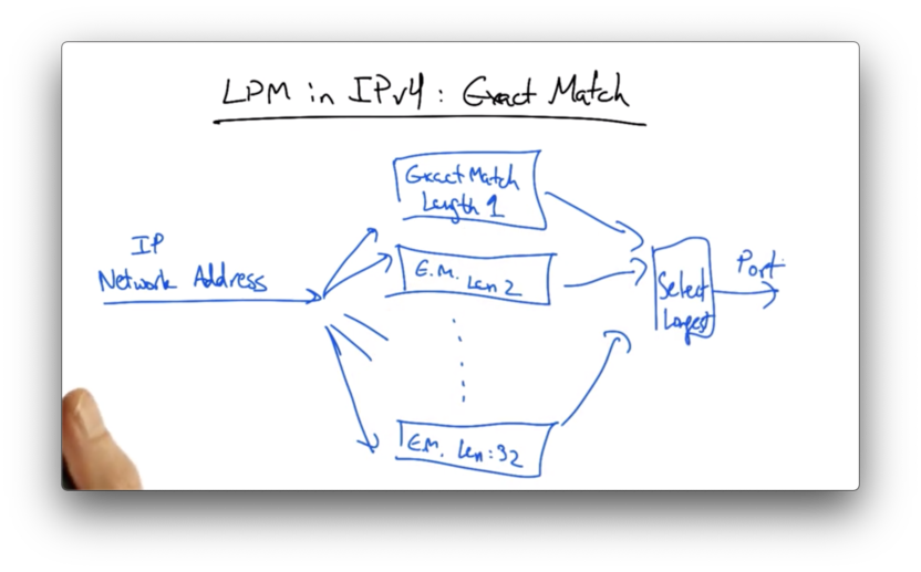
This is terribly inefficient, as we would have to maintain 32 tables, and send every network address we receive to each one of these tables.
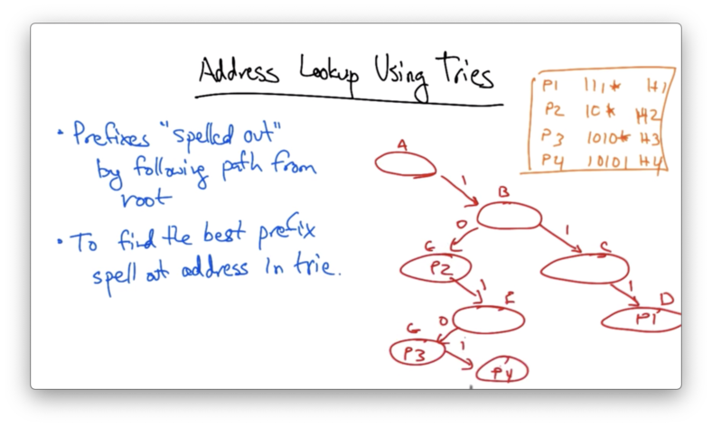
Address Lookup Using Tries
More commonly, we use a data structure called a trie to perform address lookups.
In a trie, prefixes are "spelled out" by following a path from the root. To find the best prefix, we simply spell out the address in the trie.
Lets suppose we had the prefixes in our routing table
- P1: 111*
- P2: 10*
- P3: 1010*
- P4: 10101
In a trie, spelling out the bit 1 always adds a node to the right, and spelling out the bit 1 always adds a node to the left.
Let's suppose we want to look up 10111. All we have to do is spell this out in the trie.
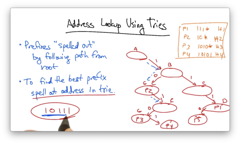
We can see that there is no entry for 1011. So we use the last node in the trie that we have traversed that has an entry. In this case, that entry is P2.
This type of trie is actually called a single-bit trie. Single-bit tries are very efficient. Every node in this trie exists as a result of the forwarding table entries that have been inserted. Put another way, this trie requires no more memory than the amount needed for all lookups. Updates are also very simple.
The main drawback of single-bit tries is the number of memory accesses that are required to perform a lookup. For a 32-bit address, looking up an address in a single bit trie may require 32 memory references in the worst case.
To put this in perspective, the OC48 spec requires no more than 4 memory accesses!
32 accesses is far too many, especially for high speed links.
Direct Trie
The other extreme is to use a direct trie where, instead of 1 bit per lookup, we might have one memory access responsible for looking up a much larger number of bits.
We might have a two-level trie, where the first memory access is dictated by the first 24 bits of the address, and the second access is dictated by the last 8 bits of the address.
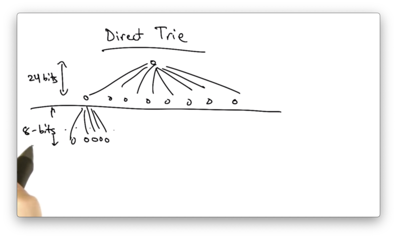
The benefit of this approach is that we can look up an entry in the forwarding table with just two accesses.
The problem with this approach is that this structure results in a very inefficient use of memory, unlike the single bit trie.
Suppose that we want to represent a /16 prefix. We have no way of encoding a lookup that is just 16 bits. We have to encode 2^8 (24 - 16) identical entries corresponding to the 2^8 /24 prefixes that are contained in the /16.
Memory Efficiency and Fast Lookup
To achieve the memory efficiency of the single-bit trie with the fast lookup properties of the direct trie, a comprise is to use a multi-bit trie, or multi-ary trie.
In a binary trie (single-bit trie), the depth is W, the degree is 2, and the stride is 1 bit.
We can generalize this in a multi-ary trie, with the depth being W/k, the degree being 2^k and the stride being k bits.
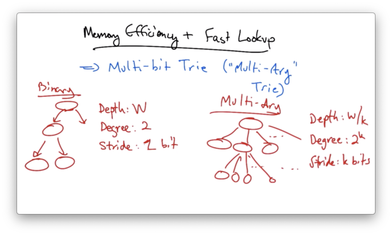
Note that the binary trie is a simple case of the multi-ary trie, where k is 1.
4-ary Trie
Let's construct a 4-ary trie (with k=2), using the same forwarding table as before.
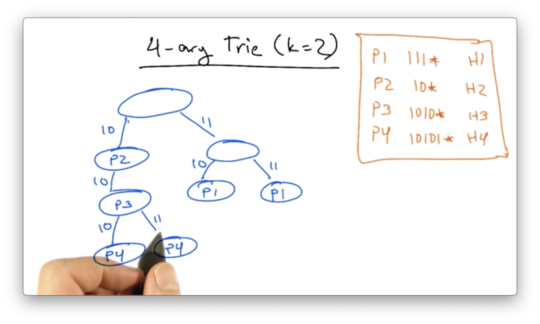
Suppose we want to again look up 10111. We can get no further than our first traversal down to P2, which is the same answer we got with the single-bit trie.
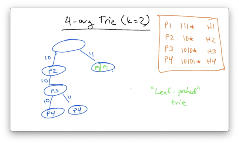
We can save space by creating a leaf-pushed trie, condensing the two P1 nodes on the right of the tree into their parent.
Other optimizations, such as Luleå and PATRICIA exist as well.
Alternatives to LPM with Tries
One alternative to implement LPM with tries is with a content-addressable memory (CAM). A CAM is a hardware-based route lookup, where there input is a tag and the output is a value. In our use case, the tag could be an IP address, and the value could be a port number.
A CAM only supports an exact match, and completes lookups in O(1).
A ternary CAM can hold three values: 0, 1 or * (wildcard). The support for a wildcard permits an implementation of LPM. One can have multiple matching entries, but prioritize the matches according to the longest non-wildcard prefix in the ternary CAM.
NAT and IPv6
The main problem that we are seeing is that IPv4 addresses only have 32 bits. This means that there can only be a total of 2^32 unique IP addresses.
Not only that, IP addresses are allocated in blocks and fragmentation of the space can mean that IPv4 address can be quickly exhausted. We have already seen the last /8 from the IPv4 address space allocated by IANA.
Two solutions to deal with this problem are network address translation and IPv6, the latter of which boasts 128-bit addresses.
Network Address Translation
Network Address Translation (NAT) allows multiple networks to reuse the same private IP address space.
A particular private IP address space that can be reused by multiple networks is 192.168.0.0/16.
Other private IP address spaces are specified in RFC 1918 (Section 3).
Obviously two networks with the same IP address cannot coexist on the public internet, because routers wouldn't know where to route a packet destined for that address.
A NAT takes a group of private IP addresses and translates it to a single, globally visible IP address for communication with the broader internet.
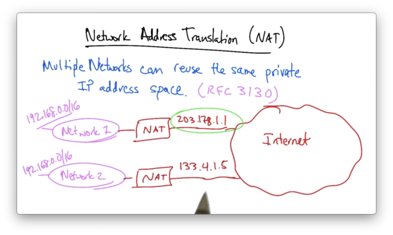
To the rest of the Internet, network 1 seems to be reachable by 203.17.1.1 and network 2 seems to be reachable by 133.4.1.5, even though both networks may use the multiple, overlapping IP addresses internally.
Say a host from network 2, such as 192.168.1.10, sends a packet destined for a global internet destination.
This packet will have source port, and the NAT will take the source IP and port and translate it to a public reachably source IP and port. The destination will remain unchanged.
For example, the packet may originally have source 192.168.1.10:1234 and the NAT may re-write this source as 133.4.1.5:5678.
The packet will make its way to the destination, and the response will re-enter the NAT at port 5678. The NAT maintains a table that maps the public IP address/port combination to a private IP address/port combination.
Thus, the NAT will rewrite the destination IP address of the packet from 133.4.1.5:5678 to 192.168.1.10:1234 and forward the packet to the originating host.
NATs are popular on broadband access networks, small/home offices, and VPNs.
There is clear savings in IPv4 address space since there can many many devices in a private network, but all of those devices "use up" only one public IP address.
The drawback to NATs is that they break the end-to-end model. If the NAT device fails, the mapping between the private IP/port and public IP/port would be lost, thereby breaking all active connections for which the NAT is on the path.
In addition, the NAT creates asymmetry. Under ordinary circumstances, it is rather difficult for a host on the global internet to reach a device in a private address space because these devices by definition do not have globally addressable IP addresses.
Thus, NATs break end-to-end communication and bidirectional communication.
IPv4 to IPv6
Another possible solution to the IP address space exhaustion problem is to simply add more bits. This is the gist of the contribution of the IPv6 protocol.
Here is the current IPv4 header.
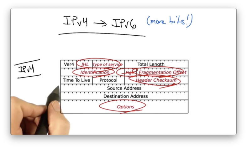
The fields in red have been removed in IPv6, leading to a much simpler header with much larger addresses.
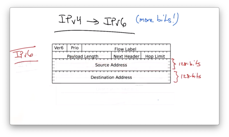
The IPv6 header provides 128 bit for both the source and destination IP address.
The format of these addresses are as follows:
The top 48 bits are for the public routing topology. The next 16 bits provide a site identifier. Finally, there is a 64 bit interface ID, which is the 48-bit Ethernet ID + 16 more bits.
The top 48 bits can be broken down even further. The top three bits are for aggregation. The next 13 bits identify the associated "tier-1" ISP. The next 8 bits are reserved, and then there are the final 24 additional bits, which are unspecified.
Note that there are13 bits in the address that directly map to the tier-1 ISP, meaning that addresses are purely provider-based. This means that changing ISPs would require renumbering.
IPv6 has many claimed benefits:
- more addresses
- simpler header
- easier multihoming
Despite these benefits, we have yet to see a huge deployment of IPv6 yet.
IPv6 Routing Table Entries
We have yet to see a significant deployment of IPv6.
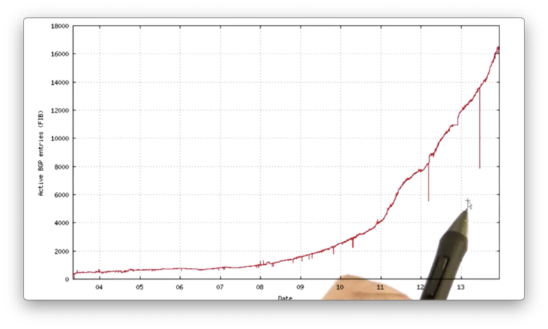
As of 2013, we have just about 16,000 IPv6 address in the global routing table, which is just a small fraction when compared to the ~500,000 IPv4 addresses present.
The problem is that IPv6 is very hard to deploy incrementally.
Remember the narrow waist. Because everything depends on the narrow waist of IPv4, and because IPv4 is built on top of so many other types of infrastructure, changing it becomes extremely tricky.
Incremental deployment, where part of the internet is running IPv4, and other parts are running IPv6, results in significant incompatibility.
IPv6 Incremental Deployment
One strategy for IPv6 incremental deployment is a dual stack deployment.
In a dual stack deployment, a host can speak both IPv4 and IPv6. It communicates with an IPv4 host using IPv4 and an IPv6 host using IPv6.
The dual stack must have an IPv4-compatible address. Either the host has both an IPv4 and IPv6 address, or it must rely on a translator which knows how to take an IPv4-compatible IPv6 address and translate it to the IPv4 address.
One possible way of ensuring compatibility of an IPv6 address with IPv4 is simply to embed the the IPv4 address in 32 bits of the 128 bits of the IPv6 address.
A dual stack host configuration solves the problem of host IP address assignment, but it doesn't solve the problem of "island" IPv6 deployments.
For example, multiple independent portions of the internet might deploy IPv6. What if the middle of the network only speaks and routes IPv4?
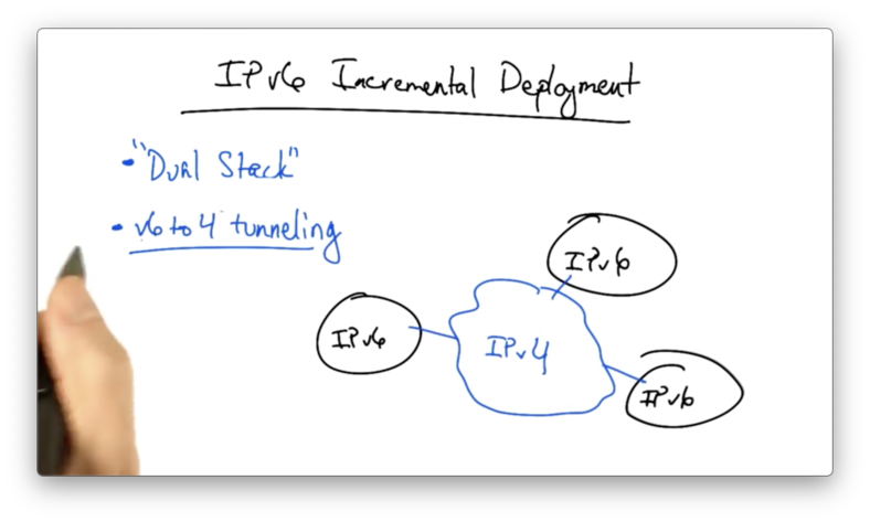
The solution is to use 6 to 4 tunneling. With this strategy, a v6 packet is encapsulated in a v4 packet.
The v4 packet is then routed to a particular v4-to-v6 gateway corresponding to the v6 address that lies behind the gateway. At this point, the outer layer of encapsulation can be stripped, and the v6 packet can be sent to its destination.
This requires the gateways at the boundaries between the v4 and v6 networks to perform encapsulation as the packet enters the v4-only part of the network, and decapsulation as the packet enters the v6 island where the destination host resides.
OMSCS Notes is made with in NYC by Matt Schlenker.
Copyright © 2019-2023. All rights reserved.
privacy policy