Congestion Control & Streaming

Congestion Control

What is congestion control and why do we need it? Simply put, the goal of congestion control is to fill the internet's "pipes" without "overflowing" them.

Congestion

Suppose that we have the following network.

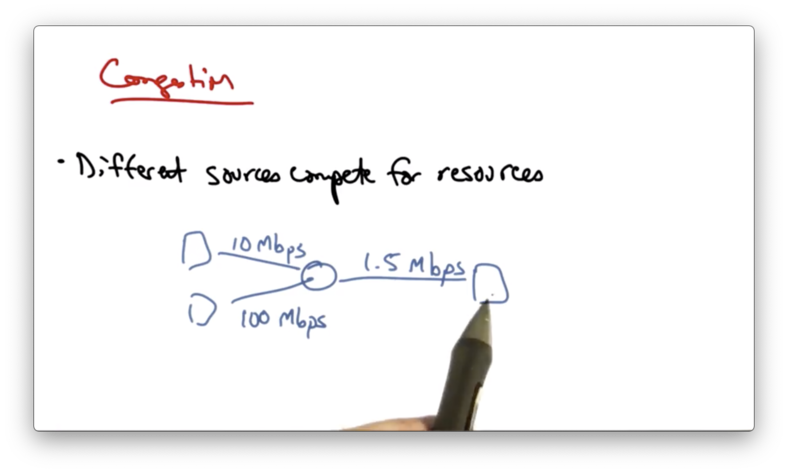
The two senders on the left can send at rates of 10Mbps and 100Mbps, respectively. The link to the host on the right, however, only has a capacity of 1.5Mbps.

The hosts on the left are competing for the same resources - capacity along the bottleneck link - inside the network.

The hosts are unaware of each other, and also of the current state of the resource they are trying to share. That is, the hosts are unaware of the amount of traffic coming from other hosts through this shared link.

Hosts that are unaware of network congestion will continue to send packets into the network, and this can result in lost packets and long delays.

Congestion Collapse

Normally, the amount of useful work done increases with the traffic load. When the network becomes saturated, the amount of useful work done plateaus: an increase in load no longer results in an increase of useful work done. After a certain point, an increase in traffic load suddenly results in a decrease in useful work done.

This decrease is known as congestion collapse.

There are many possible causes for congestion collapse.

One possibility is the spurious retransmission of packets that are still in flight. When senders don't receive acknowledgements for packets in a timely fashion, they can spuriously retransmit those packets, thus resulting in many copies of the same packets being outstanding in the network at any one time.

Another cause of congestion collapse is undelivered packets, where packets consume resources and are dropped elsewhere in the network.

Congestion control is the solution to both of these issues.

Goals of Congestion Control

Congestion control has two main goals.

The first goal is to use network resources efficiently. The second goal is to ensure that all of the senders get their fair share of the resources.

In addition, congestion control seeks to avoid congestion collapse.

Two Approaches to Congestion Control

There are two basic approaches to congestion control: end-to-end congestion control and network-assisted congestion control.

In end-to-end congestion control, the network provides no explicit feedback to the senders about when they should slow down their rates. Instead, congestion is inferred by packet loss/delay.

TCP takes the end-to-end approach to congestion control.

In network-assisted congestion control, routers provide explicit feedback about rates that end systems should be sending at.

A router might set a single bit indicating congestion, as is the case in TCP's Explicit Congestion Notification (ECN) extensions. Alternatively, a router may just explicitly specify the rate that a sender should be sending at.

TCP Congestion Control

In TCP congestion control, senders continue to increase their sending rate until they see packet drops in the network.

Packet drops occur because senders are sending at a rate that is faster than the rate at which a particular router in the network may be able to drain its buffer.

TCP interprets packet loss as congestion, and when senders see packet loss they slow down.

This is an assumption. Packet drops are not a sign of congestion in all networks. For example, in wireless networks, there may be packet loss due to corrupted packets as a result of interference.

Congestion control thus has two parts: an increase algorithm and a decrease algorithm.

In the increase algorithm, the sender must test the network to determine whether the network can sustain a higher sending rate.

In the decrease algorithm, the senders react to congestion to achieve optimal loss rates, delays and sending rates.

Two Approaches to Adjusting Rate

Window Based

One approach is a window-based algorithm. In this approach, a sender can only have a certain number of packets outstanding, or "in flight".

The sender uses acknowledgements from the receiver to clock the retransmission of new data.

Suppose the sender's window is four packets.

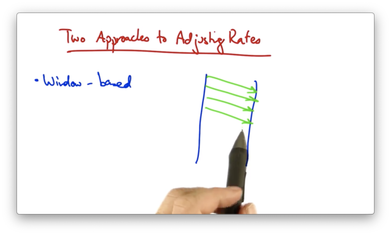
At this point, there are four packets outstanding in the network, and the sender cannot send more packets until it has received an acknowledgement from the receiver.

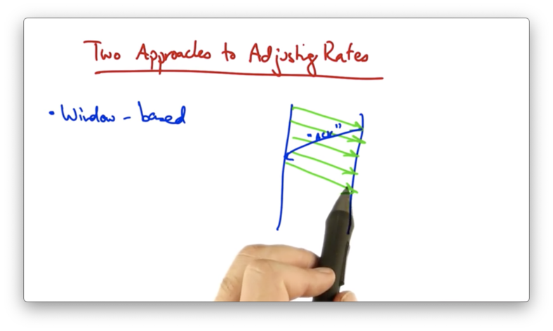
When the acknowledgement is received, the sender can send another packet. Thus, there are still four packets in flight after the first "ACK" has been received.

If a sender wants to increase the rate at which it is sending, it simply needs to increase its window size.

In TCP, the sender increases its window size by one for every ACK that it receives. In this example, once the first packet is ACKed, the sender may send two additional packets, increasing its window size to five.

This is called additive increase.

If a packet is not acknowledged, the window size is cut in half. This is called multiplicative decrease.

TCP's congestion control is called additive increase, multiplicative decrease (AIMD).

Rate Based

Another approach is a rate-based algorithm. In this case, the sender monitors the loss rate, and uses a timer to modulate the transmission rate.

Fairness and Efficiency in Congestion Control

The two goals of congestion control are fairness and efficiency.

Fairness means that everyone gets their fair share of the network resources.

Efficiency means that the network resources are used well. We shouldn't have a case where there is spare capacity in the network and senders have data to send but are unable to do so.

We can represent fairness and efficiency in terms of a phase plot where each axis represents a particular sender's allocation.

Suppose we have two users in the network, and their sending rates are x1 and x2. If the capacity of the network is C, then we can represent the full utilization of the network as the line x1 + x2 = C.

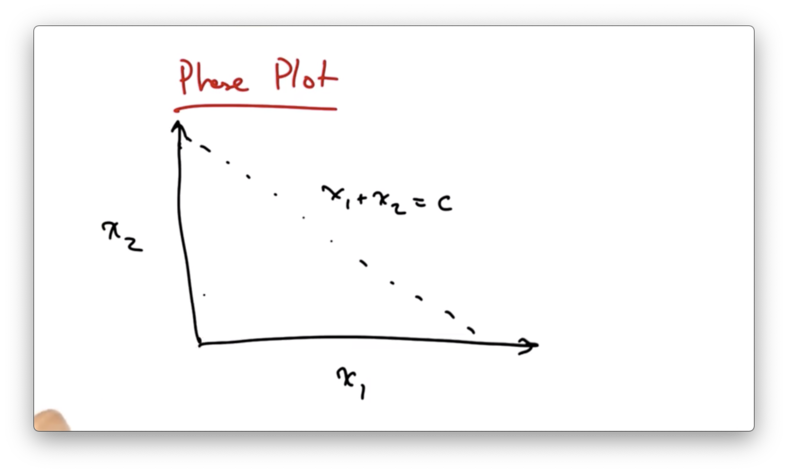
Anything to the left of this line represents under utilization of the network, and anything to the right of this line represents over utilization of the network.

We can also represent "fairness" as the line x1 = x2.

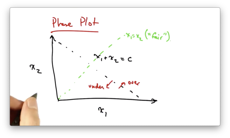
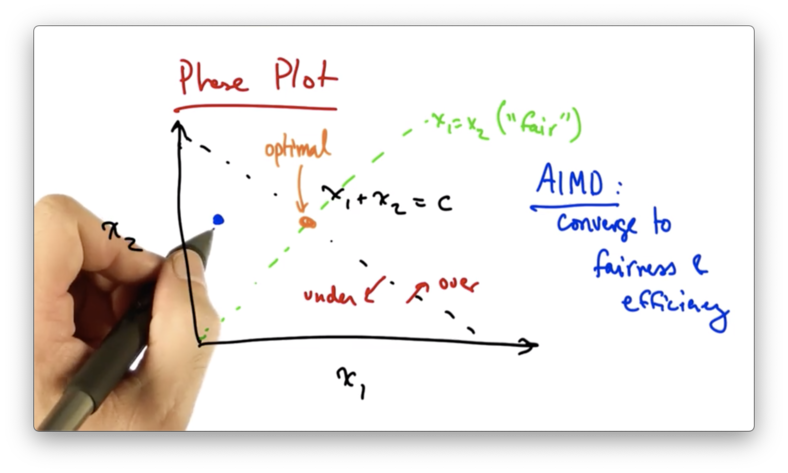
The optimal network resource allocation in this case is the intersection of the two lines; namely, where both senders have equal rates that utilize the network completely.

We can use this phase diagram to understand why senders who use AIMD converge to the optimal operating point.

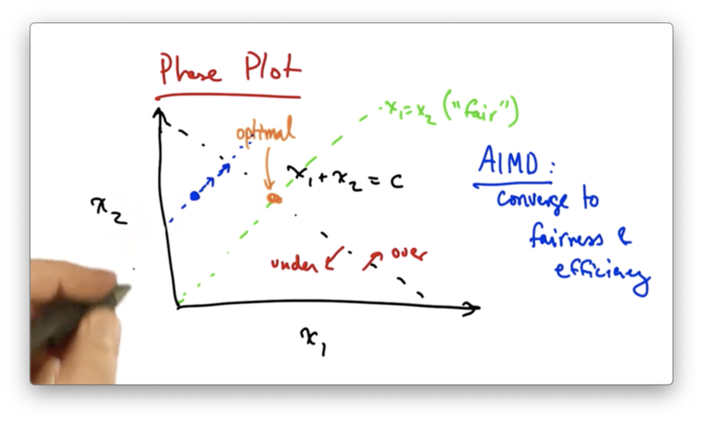
Let's suppose that we start at the following operating point.

At this point, both senders will additively increase their sending rates. This results in moving along a line that is parallel to the line x1 = x2 since both senders are increasing their rate by the same amount.

Additive increase will continue until the network becomes overloaded.

At this point, the senders will see a packet drop and perform multiplicative decrease, cutting their rates by some constant factor.

This new operating point will fall closer to the line of "fairness".

At this point, both senders will additively increase their sending rates again. This results in moving along a line that is parallel to the line x1 = x2 since both senders are increasing their rate by the same amount.

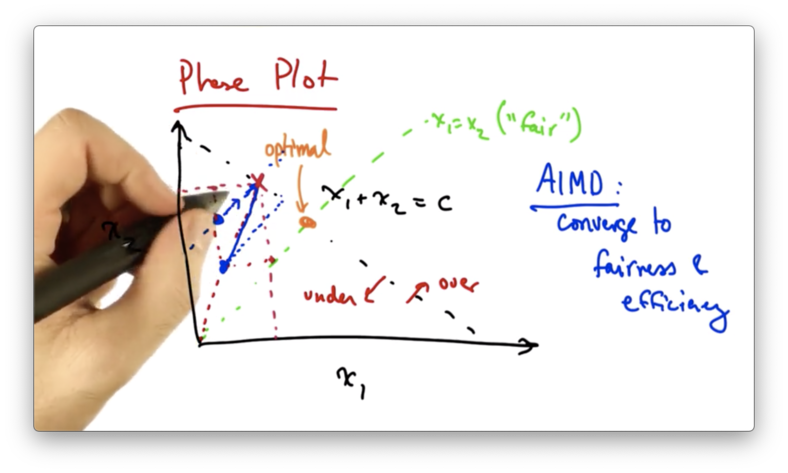
Eventually, the senders will reach the optimal operating point.

Every time that additive increase is applied, the senders move toward efficiency. Every time that multiplicative decrease is applied, the senders move toward fairness.

AIMD

The additive increase, multiplicative decrease algorithm is distributed, fair and efficient.

To visualize the sender's sending rate over time, we can look at a TCP sawtooth, which plots the congestion window over time.

This particular diagram plots the congestion window (in packets) over time (in RTTs).

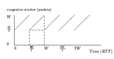
TCP periodically probes for available bandwidth by increasing its congestion window using additive increase.

When the sender reaches a saturation point by filling up a buffer in a router somewhere along the path, it will see a packet drop. At this point, the sender will decrease its congestion window by half.

The average congestion window, given the maximum window size of W - right before the drop - and the minimum of W/2 - right after the drop - is 3W/4, the halfway point.

In order to increase the window size by 1, we must wait for 1 packet acknowledgement to come back. Thus, each additive increase in the congestion window takes 1 RTT. The increase from the window size W/2 to W takes W/2 (W - W/2 ) RTTs.

The number of packets transmitted between instances of packet loss can be calculated by taking the area under the sawtooth, outlined in dotted lines in the figure above.

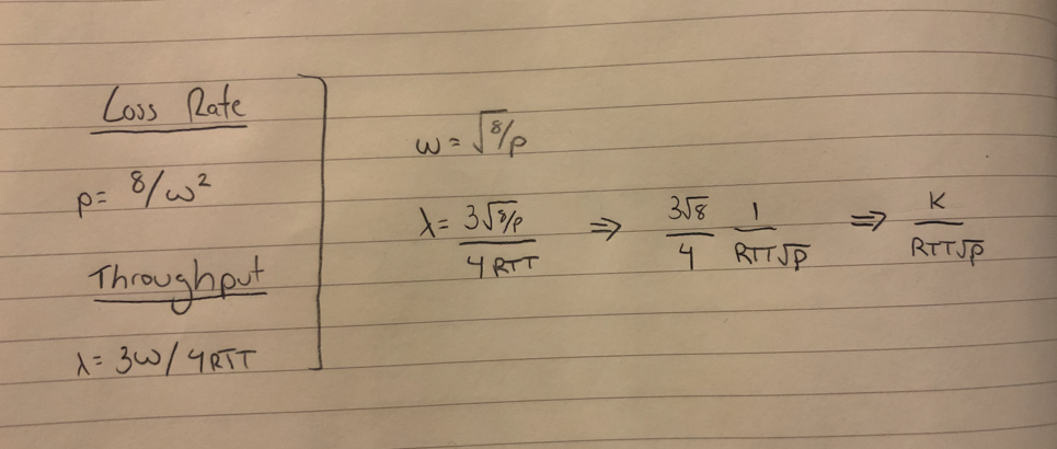
In this case, we have (W/2)^2 + ((W/2)^2) / 2. The video ignores the first term, so we can send (W/2)^2 / 2, or W^2 / 8 packets for every packet that we drop. Our actual loss rate is 1 over this quantity, or 8 / W^2.

We can calculate the throughput of the sender by taking the average window size and dividing by the round trip time. Thus, the throughput of the sender is 3W / 4RTT.

If we want to relate the throughput to the loss rate

Data Centers and TCP Incast

A typical data center consists a set of server racks - each holding a large number of servers - the switches connecting those racks, and the connecting links that connect those switches to other parts of the topology.

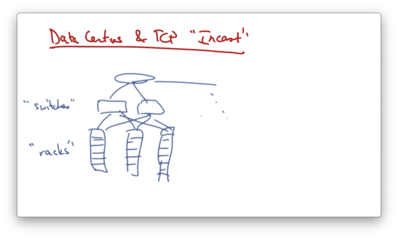
One characteristic of a data center is a high fan-in: there are many leaves (servers) relative to the higher layers in the tree (switches).

Workloads in a datacenter are high bandwidth and low latency. Many clients issues requests in parallel, each with a relatively small amount of data per request.

In addition, the buffers in data center switches can be quite small.

The throughput collapse that results from this combination is called the TCP incast problem.

Incast is a drastic reduction in application throughput that results when servers using TCP all simultaneously request data, leading to a gross underutilization of network capacity in many-to-one communication networks, like a datacenter.

The filling up of the buffers at the switches result in bursty retransmissions that overfill the switch buffers. These bursty retransmissions are caused by TCP timeouts.

Roundtrip times in a datacenter are often just hundreds of microseconds, but TCP timeouts can last hundreds of milliseconds. Because RTT is so much less than timeouts, senders will have to wait for TCP timeout before they retransmit, which can reduce application throughput by as much as 90%.

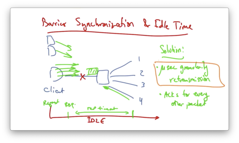
Barrier Synchronization and Idle Time

A common request pattern in datacenters today is barrier synchronization, whereby a client may have requests issued from many parallel threads and no forward progress can be made until all the responses for those threads are satisfied.

For example, a client might send a synchronized read with four parallel requests. Suppose that the fourth request is dropped.

We have a request that is issued at time 0, and response that comes back for threads 1-3 100us later. TCP might timeout on the fourth. In this case, the link is idle for a very long time until the fourth connection times out.

The addition of more clients in the network induces an overflow of the switch buffer, causing severe packet loss, inducing throughput collapse.

One solution to this problem is to use fine-grained TCP retransmission timers, on the order of microseconds instead of milliseconds.

This would reduce the retransmission timeout for TCP, which would improve the system throughput.

Another way to reduce the network load is to have the client acknowledge every other packet, instead of every packet.

Multimedia and Streaming

In this section we will talk about

• digital audio and video data
• multimedia applications
• multimedia transfers over best-effort networks
• quality of service

Some multimedia applications that we use today include

• youtube
• skype
• google hangouts

Challenges

One challenge is that there is a large volume of data. Each sample is a sound or an image and there are many samples per second.

Sometimes, because of the way the data is compressed, the volume of data that is being sent may vary over time. The data may not be sent at a constant rate, yet in streaming we want smooth layout.

Users typically have a very low tolerance for delay variation. It's very annoying for a video to stop after it has started playing.

Users might have a low tolerance for delay, period. Consider your tolerance for delay when playing an online game or using a VoIP application.

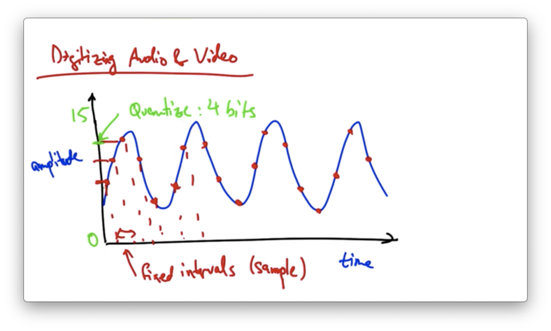
Digitizing Audio and Video

Suppose we have an analog audio signal that we would like to digitize - convert to a stream of bits.

We can sample the audio signal at fixed intervals and represent the amplitude of each sample with a fixed number of bits.

For example, if our dynamic range was from 0 to 15, we could quantize the amplitude of the signal such that each sample could be represented with 4 bits.

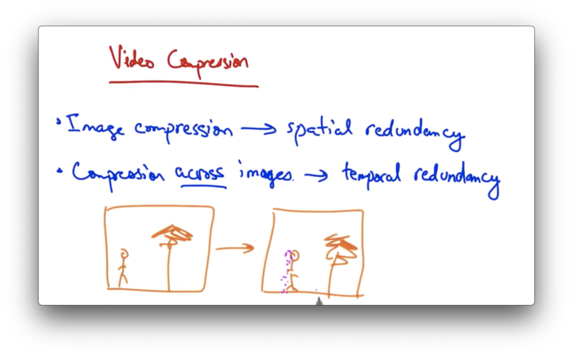
Video Compression

A video is a sequence of images.

Spatial redundancy allows us to compress a single image. Temporal redundancy allows us to perform compression across images.

For example, if a person is walking towards a tree, two consecutive images might be almost the same except for the person, who will be in a slightly different position.

Video compression uses a combination of static image compression on reference/anchor (I) frames and derived (P) frames.

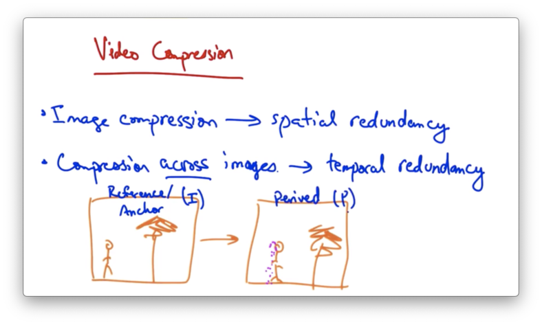
If we take the I frame and divide it into blocks, we can then see that the P frame is almost the same except for a few blocks that can be represented in terms of the original iframe blocks plus a few motion vectors.

A common video compression format used on the internet is MPEG.

Streaming Video

In a streaming video system, the streaming server stores the audio and video files, and the client requests the files and plays them as they download.

It's important to play the data at the right time.

The server can divide the data into segments and then label each segment with a timestamp indicating the time at which that particular segment should be played. This ensures that the client knows when to play that segment.

The data must arrive at the client quickly enough; otherwise, the client can't keep playing.

The solution is to have the client use a playout buffer where the client stores data as it arrives from the server, and plays the data for the user in a continuous fashion.

Data might arrive more slowly or more quickly from the server, but as long as the client is playing data out of the buffer at a continuous rate, the user sees a smooth playout.

A client may typically wait a few seconds before playing a stream to allow data to be built up in the buffer. This helps to account for times when the server is not sending data at a rate that is sufficient to satisfy the client's playout rate.

Playout Delay

The rate at which packets are generated does not necessarily equal the rate at which packets are received.

Network traffic may introduce variable delay in packet transmission from the server to the client.

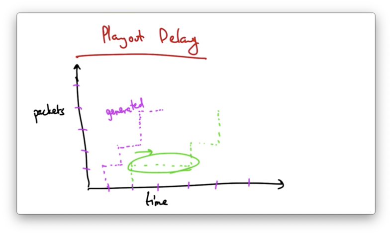
We want to avoid these types of delays when we play out.

If we first wait to receive several packets in order to fill the buffer before we start playing, then we can have a playout schedule that is smooth regardless of the erratic arrival times that may result from network delays.

Some delay at the beginning of the play out is acceptable: users can typically tolerate startup delays of a few seconds.

Clients cannot tolerate high variation in packet arrival if the buffer starves.

In addition, a small amount of loss/missing data does not disrupt the playback, but retransmitting a lost packet might take too long, resulting in unacceptable delays.

TCP is Not a Good Fit

TCP is not a good fit for congestion control for streaming audio/video.

TCP retransmits lost packets but retransmissions in the context of streaming media may not always be useful.

TCP also slows down its sending rate after packet loss, which may cause starvation of the client.

As well, TCP as a protocol contains a certain amount of overhead. A TCP header of 20 bytes on every packet is large for audio samples. Sending acknowledgements for every other packet may be more feedback than is needed.

Instead of TCP, one might consider the User Datagram Protocol (UDP), which does not retransmit lost packets and does not automatically adjust its sending rate. UDP also has a smaller header.

Because UDP does not retransmit lost packets or adjust its sending rate, many things are left to higher layers. For example, the sender must still ensure that the sending rate is friendly to other TCP senders that may be sharing the link.

There are a variety of audio/video streaming transport layer protocols that are built on top of UDP that allow senders to figure out how and when to retransmit packet and how to adjust their sending rates.

More Streaming

YouTube

With YouTube, all uploaded videos are converted to flash. Since most modern browsers contain a flash plugin, the browser can easily play these videos.

Communication between the browser and YouTube occurs over HTTP/TCP. Even though TCP is suboptimal for streaming applications, the designers of YouTube decided to keep things simple, potentially at the expense of video quality.

When a client makes an HTTP request to youtube.com, the request is redirected to a Content Distribution Network (CDN) server. When the client sends the request to the CDN server, the server responds with the video stream.

Skype/VoIP

With Skype and VoIP, the analog voice signal is digitized through an A/D conversion, and this resulting bit stream is sent over the internet.

In the case of Skype, the A/D conversion happens by way of the application.

In the case of VoIP, the conversion will be performed be a phone adapter that you physically connect to your phone. An example of such an adapter is Vonage.

The adapter sends and receives data packets and then communicates with the phone in a standard way.

Skype is based on peer-to-peer (P2P) technology, where individual users route voice traffic through one another.

Skype

Skype has a central login server but then uses P2P to exchange the actual voice streams.

Skype compresses the audio to achieve a fairly low bitrate. At 67 bytes per packet and 140 packets per second, Skype uses about 40 kilobits per second in each direction.

While good data compression and direct P2P communication are helpful in improving the quality of the audio, the network ultimately plays a large role in quality.

Long propagation delays, high congestion, and disruptions can all degrade the quality of a VoIP call.

To ensure that some streams achieve acceptable performance levels, we sometimes perform Quality of Service (QoS).

One way to perform QoS is by marking certain packet streams as higher priority than others.

Marking and Policing

Applications compete for bandwidth.

Consider a VoIP application and an FTP application that are sharing the same link.

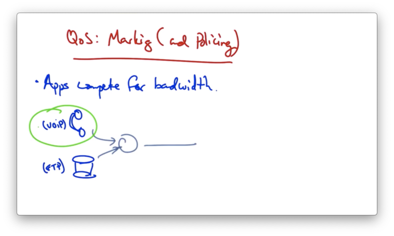
We'd like the audio packets to receive priority over the file transfer packets since the user's experience can be significantly degraded by lost or delayed audio packets.

We want to mark the audio packets as they arrive at the router so that they receive a higher priority than the file transfer packets.

You could imagine implementing this using priority queues, with the VoIP packets being placed in a higher priority queue than the FTP packets.

An alternative to priority queueing is to allocate fixed bandwidth per application. The problem with this alternative is that it can result in inefficiency if one of the flows doesn't fully utilize its fixed allocation.

In addition to marking and policing, the router must apply scheduling.

One strategy for scheduling is weighted fair queueing, where the queue containing the VoIP packets is served more frequently than the queue containing the FTP packets.

Another alternative is to use admission control, whereby an application declares its needs in advance and the network may block the application's traffic if the network can't satisfy the application's needs.

A busy signal on a telephone network is an example of admission control.

The user experience that results from blocking in admission control is one of the reasons that admission control is not frequently used in internet applications.