Kalman Filters

Tracking Intro Quiz

In the last lesson, we talked about localization, the process by which we could use sensor data to provide an estimation of a robot's location in the world.

In this lesson, we concern ourselves with finding other moving objects in the world. We need to understand how to interpret sensor data to understand not only where these other objects are but also how fast they are moving so that we can move in a way that avoids collisions with them in the future. The technique that we are going to use to solve this problem, known as tracking, is the Kalman filter.

This method is very similar to the Monte Carlo localization method we discussed in the previous lesson. The primary difference between the two is that Kalman filters provide estimations over a continuous state, whereas Monte Carlo localization required us to chop the world into discrete locations. As a result, the Kalman filter only produces unimodal probability distributions, while the Monte Carlo method can produce multimodal distributions.

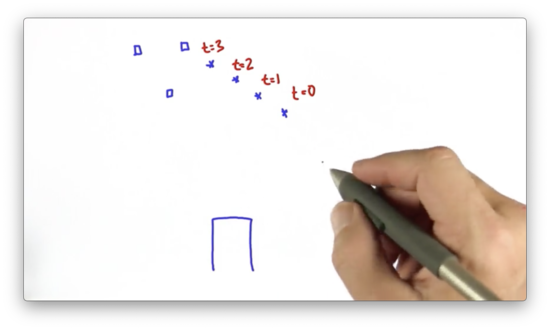
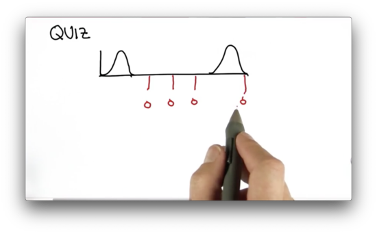
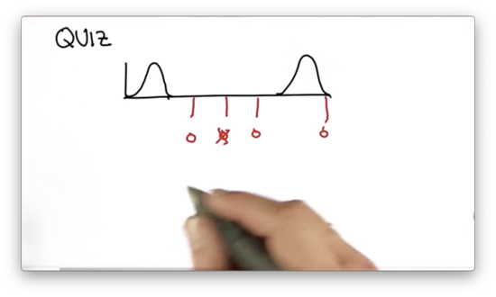
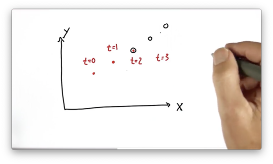
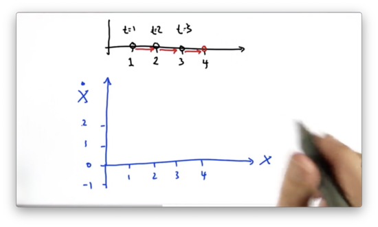
Let's start with an example. Consider a car driving along in the world. Let's assume this car senses an object, represented by an "*" below, in the depicted locations at times $t=0$, $t=1$, $t=2$, and $t=3$. Where is the object going to be at time $t=4$?

Tracking Intro Quiz Solution

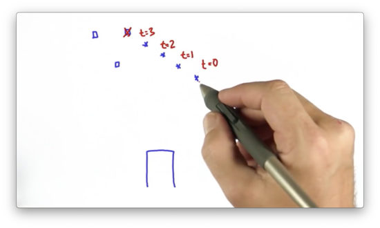
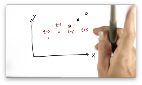
From the positional observations thus far, as well as the corresponding timestamps, we can intuitively infer the velocity of the object "*". At time $t=4$, we expect the object, barring any drastic change in velocity, to move roughly the same distance, in roughly the same direction, as it has in the past.

Kalman filters allow us to solve precisely these types of problems: estimating future locations and velocities based on positional data like this.

Gaussian Intro Quiz

When we talked about localization in the last lesson, we sliced the world into a finite number of grid cells and assigned a probability to each grid cell.

Such a representation, one that divides a continuous space into a set of discrete locations, is called a histogram. Since the world is a continuous space, our histogram distribution is only an approximation of the underlying continuous distribution.

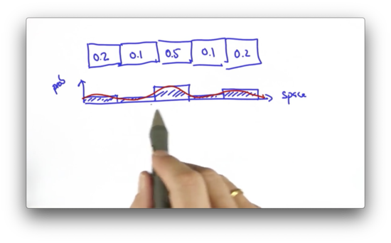
In Kalman filters, the probability distribution is given by a Gaussian. A Gaussian is a continuous function over a space of inputs - locations, in our case. Like all probability distributions, the area underneath a Gaussian equals one. Furthermore, a Gaussian is characterized by two parameters: a mean, $\mu$, and a variance, $\sigma^2$.

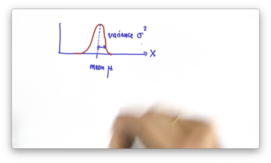
Since a Gaussian is a continuous function, there is no histogram to maintain as we sense and move. Instead, our task is to maintain a $\mu$ and $\sigma^2$ that parameterize the Gaussian that serves as our best estimate of the location of the object that we are trying to localize.

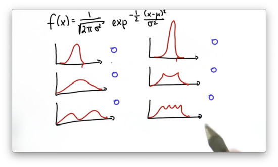
The formula for a Gaussian function, $f(x)$ is an exponential of a quadratic function:

where $\exp(x) = e^x$.

If we look at the expression inside the exponential, we can see that we are taking the squared difference of our query point, $x$, and our mean, $\mu$, and dividing this squared difference by the variance, $\sigma^2$.

If $x = \mu$, the numerator in this expression becomes zero, so we have $\exp(0) = 1$. This result makes intuitive sense, as the probability should be maximal when $x$ equals the mean of the distribution.

This observation, that $f(\mu) = 1$, might seem puzzling. If $f(x)$ is to be a valid probability distribution, then it must return 0 for all $x \neq \mu$. To reconcile this issue, the complete formula for the Gaussian function actually includes a normalization factor:

However, for everything we are going to talk about regarding Kalman filters, this constant doesn't matter, so we can ignore it.

Let's look at a quiz now. Given the following functions, which ones do you think are Gaussians?

Gaussian Intro Quiz Solution

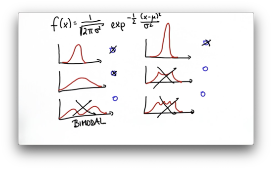
One prominent characteristic of Gaussian functions is that they are unimodal; that is, they have a single "peak". The third, fifth, and sixth functions are all multimodal, so they cannot be Gaussians.

Variance Comparison Quiz

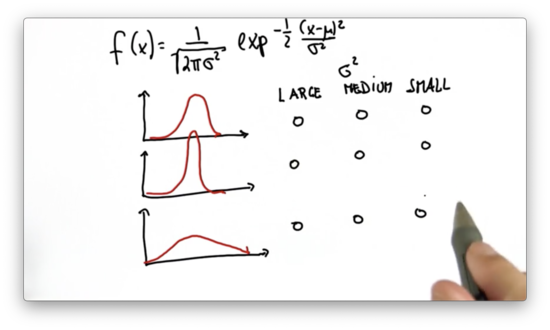
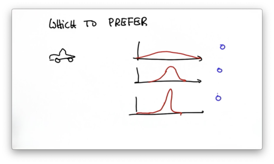
Given the following graphs of three different Gaussians, which one has the large variance, the medium variance, and the small variance?

Variance Comparison Quiz Solution

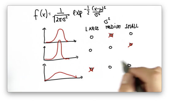
The difference between $x$ and $\mu$ is normalized by $\sigma^2$. Larger values of $\sigma^2$ penalize large differences between $x$ and $\mu$ less than smaller values. As a result, Gaussians with large variances produce larger values of $f(x)$ when $x$ is far from the mean than do Gaussians with smaller variances.

Another way to think about it is that variance is a measure of uncertainty. For example, the third Gaussian has the highest variance and the lowest probability associated with its mean value. On the other hand, the second Gaussian has the smallest variance and, therefore, the highest probability associated with its mean value.

Gaussians parameterized by larger variances spread probability over a larger number of possibilities, while those with smaller variances concentrate probability over a smaller number of possibilities.

Preferred Gaussian Quiz

If we are tracking another car from within our car, which Gaussian would we prefer to see as an estimate of the other car's location?

Preferred Gaussian Quiz Solution

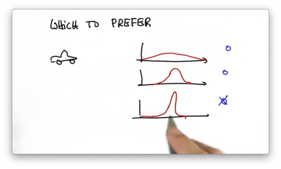
Because the third Gaussian has the smallest variance, it represents the most certain estimate of the other car's location. The more certain we can be about where another car is located, the more confidently we can maneuver to avoid hitting it.

Evaluate Gaussian Quiz

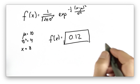
Given a Gaussian, $f(x)$, parameterized by $\mu = 10$ and $\sigma^2 = 4$, what is $f(8)$? As a reminder, here is the formula for the Gaussian we use:

Evaluate Gaussian Quiz Solution

Maximize Gaussian Quiz

We have the following python function, f, which takes as input mu, sigma2 and x, and returns the output of the Gaussian function, parameterized by mu and sigma2, for x.

Given mu = 10 and sigma2 = 4, what value of x can we pass into f to maximize the returned value?

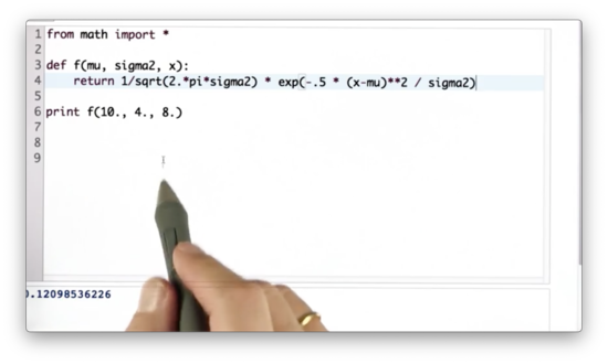
Maximize Gaussian Quiz Solution

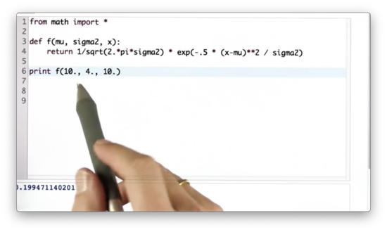
If we set x equal to mu, then we maximize the exponential expression in the Gaussian function, as exp(-0.5 * 0) = exp(0) = 1. As a result, we maximize the function overall, since the normalization factor is a constant.

Measurement and Motion 1 Quiz

When we talked about localization, we talked about manipulating our probability distributions via measurement updates and motion updates. We can apply this exact iterative adjustment when working with Kalman filters as well.

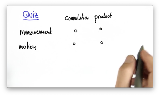
Let's see if we remember from the localization lectures. Does the measurement update involve a convolution or a product? What about the motion update?

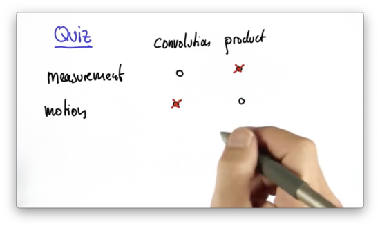
Measurement and Motion 1 Quiz Solution

Measurement and Motion 2 Quiz

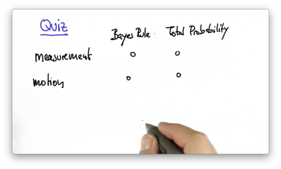
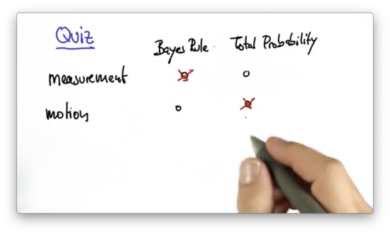
Let's see if we remember from the localization lectures. Does the measurement update involve Bayes' rule or the theorem of total probability? What about the motion update?

Measurement and Motion 2 Quiz Solution

Shifting the Mean Quiz

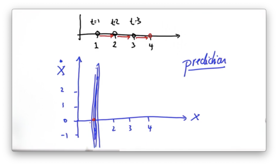
When using Kalman filters, we iterate between measurement and motion. The measurement update uses Bayes' rule, which produces a new posterior distribution by taking the product of the prior distribution and the information we gain from our measurement. The motion update - also known as the prediction - uses the theory of total probability, which produces a new posterior by adding the motion to the prior.

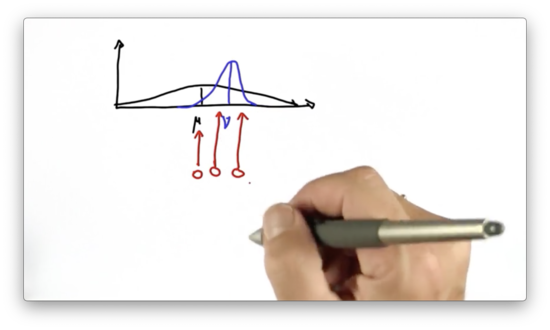
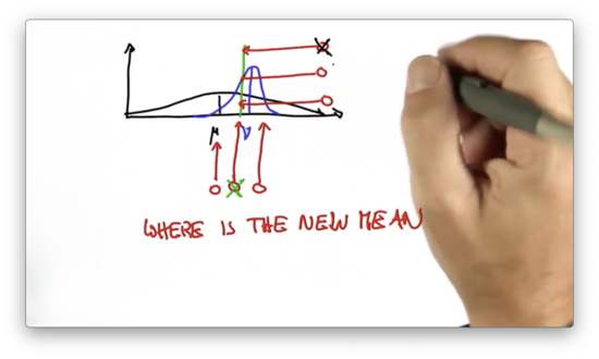
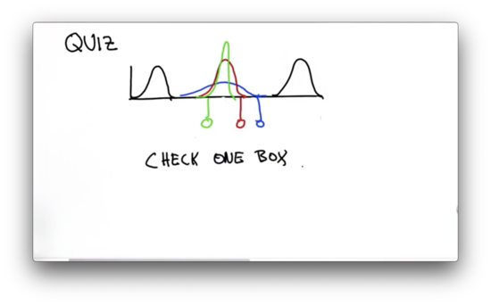
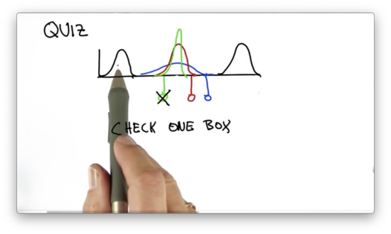
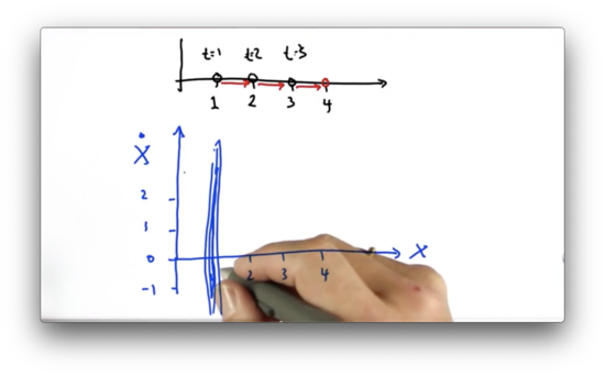
Suppose we are localizing another vehicle, and we have the following prior distribution, shown in black below. Note that this Gaussian is very wide, indicating a high level of uncertainty about the position of the vehicle.

Suppose now we take a measurement which gives us an updated distribution on the position of the vehicle, shown in blue before. Note that this Gaussian is quite narrow, indicating a large increase in certainty regarding the position of the vehicle.

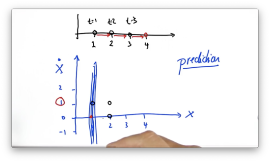
We have to combine the two distributions to produce our posterior distribution. Which of the three red lines below corresponds to the mean of our posterior distribution?

Shifting the Mean Quiz Solution

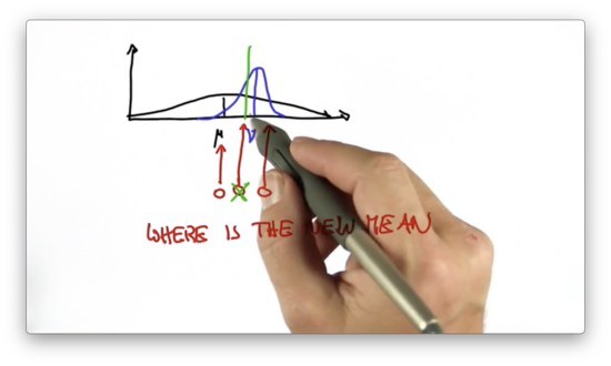
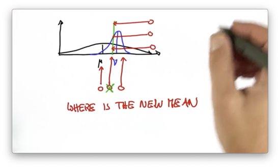
The mean of the resulting posterior distribution lies in between the mean of the prior and the mean of the distribution as given by the measurement. Note that the new mean lies slightly closer to the mean of the measurement-based distribution since that distribution is more certain of the location of the vehicle than was the prior. The more certain we are, the more we pull the mean in the direction of the certain answer.

Predicting the Peak Quiz

We've found the location of the mean of the posterior distribution. Now let's focus on the "peakiness" of this distribution.

We can think about "peakiness" in two different ways. First, peakiness is inversely related to variance. The measurement-based distribution, which has a smaller variance, has a higher peak than the prior.

We can also think about peakiness as a visual representation of certainty since we know that we can use variance as a measure of certainty. Indeed, the prior is less certain about the vehicle location than is the measurement-based distribution and, therefore, has a smaller peak.

Given this information, how high should we expect the peak of the resulting distribution to be? Below the peak of the prior, above the peak of the measurement-based distribution, or somewhere in the middle?

Put another way, is our posterior: more confident than the constituent distributions, less confident, or somewhere in between?

Predicting the Peak Quiz Solution

Very surprisingly, the posterior distribution is more certain - has a higher peak - than either of the two component distributions. The variance of this distribution is smaller than both that of the prior distribution and the measurement-based distribution.

Parameter Update Quiz

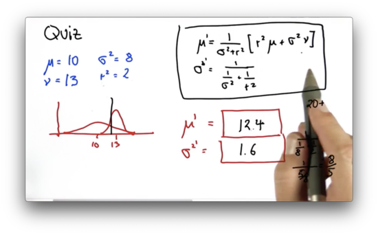
Suppose we have two Gaussians - the prior distribution and the measurement probability - and we want to multiply them using Bayes' rule to produce a posterior distribution. The prior has a mean $\mu$ and a variance $\sigma^2$, while the measurement probability has a mean $\nu$ and a variance $r^2$.

The new mean, $\mu^\prime$, is the weighted sum of the old means, where $\mu$ is weighted by $r^2$ and $\nu$ is weighted by $\sigma^2$. This sum is normalized by the sum of the weighting factors: $r^2 + \sigma^2$.

The new variance term, $\sigma^{2\prime}$, is given by the following equation.

Let's put this into action using the prior distribution and measurement probability we have been examining.

Clearly, the prior distribution has a much larger uncertainty than the measurement probability. Thus, $\sigma^2 > r^2$, which means that $\nu$ is weighted more heavily than $\mu$ in the calculation of $\mu^\prime$. As a result, $\mu^\prime$ sits closer to $\nu$, than $\mu$, which is consistent with what we have seen.

Interestingly, the variance calculation is unaffected by the previous means and only considers the previous variances. The resulting variance is always larger than both $r^2$ and $\sigma^2$.

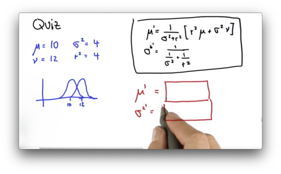
Suppose we have two Gaussians: one parameterized by $\mu = 10$ and $\sigma^2 = 4$, and another parameterized by $\nu = 12$ and $r^2 = 4$. What are the values of $\mu^\prime$ and $\sigma^{2\prime}$ as a result of the measurement update?

Parameter Update Quiz Solution

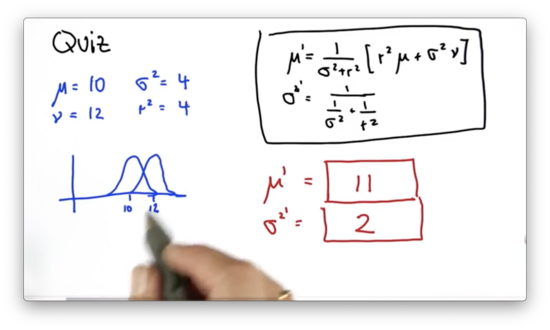
We can calculate the new mean, $\mu^\prime$, as follows.

Note that because $r^2 = \sigma^2$, the normalized weighted average of $\mu$ and $\nu$ is equivalent to the arithmetic average: $\frac{\mu + \nu}{2}$.

We can calculate the new variance, $\sigma^{2\prime}$, as follows.

We may have been surprised earlier that the variance of the posterior distribution was smaller than the variance of both the prior and the measurement probability. Here we have demonstrated that fact mathematically.

Parameter Update 2 Quiz

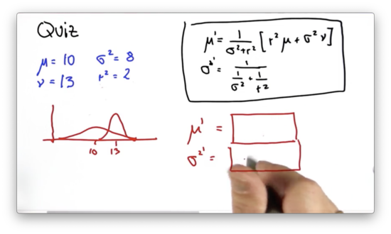
Suppose we have two Gaussians: one parameterized by $\mu = 10$ and $\sigma^2 = 8$, and another parameterized by $\nu = 13$ and $r^2 = 2$. What are the values of $\mu^\prime$ and $\sigma^{2\prime}$ as a result of the measurement update?

Parameter Update 2 Quiz Solution

We can calculate the new mean, $\mu^\prime$, as follows.

As we expect, $\mu^\prime$ is much closer to $\nu$ than $\mu$, since $\sigma^2$ is much larger than $r^2$.

We can calculate the new variance, $\sigma^{2\prime}$, as follows.

Again, we can see that the resulting variance is less than that of either of the component distributions.

Separated Gaussians Quiz

Suppose we have the following prior distribution and measurement probability, each with the same variance. Which of the following positions - marked in red below - corresponds to the mean of the posterior distribution produced by combining these two distributions?

Separated Gaussians Quiz Solution

Since the two variances are the same, the new mean is simply the arithmetic average of the means of the two component distributions.

Separated Gaussians 2 Quiz

Suppose we have the following prior distribution and measurement probability, each with the same variance. Which of the following Gaussian represents the combination of the two? There are three choices: a Gaussian with a larger variance than the two component distributions, a Gaussian with an equivalent variance, and a Gaussian with a smaller variance.

Separated Gaussians 2 Quiz Solution

As we have seen from the math, the resulting Gaussian has a smaller variance - that is, it is more peaky - than the component distributions. We can again demonstrate this fact using the equation for the new variance, $\sigma^{2\prime}$. Remember that both component Gaussians have the same variance.

New Mean and Variance Quiz

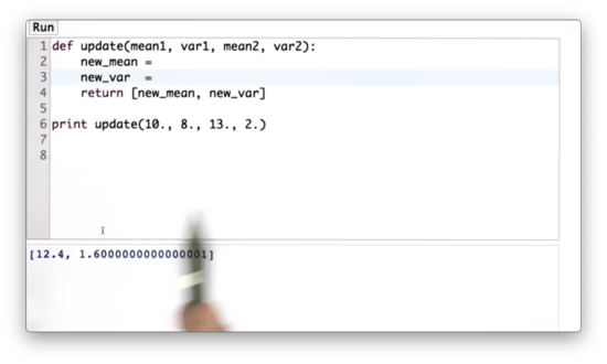
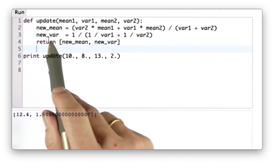
Given the following python function, update, which takes as input the means and variances of two Gaussians - mean1, var1, and mean2, var2, respectively - our task is to write some code that computes new_mean and new_var according to the update rules we have been working with so far.

New Mean and Variance Quiz Solution

Gaussian Motion Quiz

Suppose we live in a world where the following Gaussian represents our best estimate as to our current location.

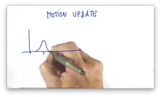
Now suppose we issue a motion command to move to the right a certain distance. We can think about the motion as being represented by its own Gaussian, having an expected value, $u$, and an uncertainty, $r^2$.

We can combine the motion with the prior to produce our prediction, parameterized by $\mu^\prime$ and $\sigma^{2\prime}$ as follows.

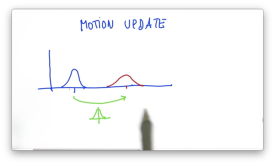
Intuitively, this makes sense. If we expect to move to the right by $u$, then it makes sense that we shift our mean by exactly $u$. Additionally, since we have uncertainty in the prior and uncertainty in the motion, we can expect that our prediction has even more uncertainty than either of the two component Gaussians.

Let's take a quiz now. Suppose we have a Gaussian before the movement, parameterized by $\mu = 8$ and $\sigma^2 = 4$. We issue a motion command with an expected value $u = 10$ and uncertainty $r^2$. What are the parameters, $\mu^\prime$ and $\sigma^{2\prime}$ of the predicted Gaussian?

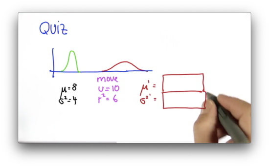
Gaussian Motion Quiz Solution

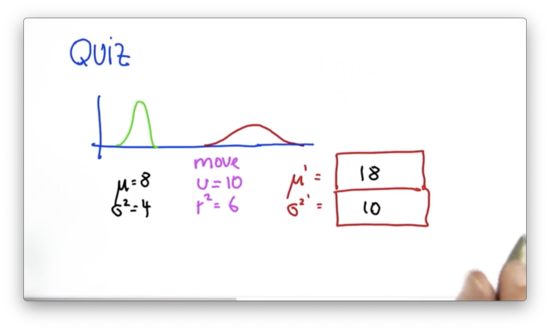
Remember the following equations.

Predict Function Quiz

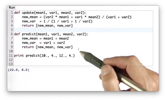
Given the following python function, predict, which takes as input the means and variances of two Gaussians - mean1, var1, and mean2, var2, respectively - our task is to write some code that computes new_mean and new_var according to the prediction rules we have been working with so far.

Predict Function Quiz Solution

Kalman Filter Code Quiz

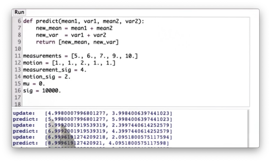
Let's write a main program that takes these two functions, update and predict, and feeds into them an alternating sequence of measurements and motions.

The measurements we are going to use are measurements = [5,6,7,9,10] and the motions are motions = [1,1,2,1,1]. Our initial belief as to our position is a Gaussian parameterized by mu = 0 and a very large uncertainty sig = 10000.

Furthermore, the measurement uncertainty, measurement_sig, is constant and equal to 4, while the motion uncertainty, motion_sig, is constant and equal to 2.

Kalman Filter Code Quiz Solution

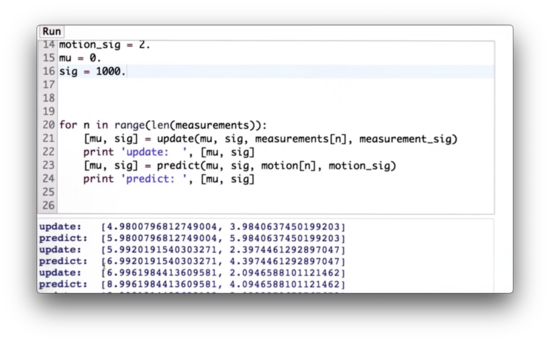
We iterate through the measurements and motions updating mu and sig first according to the rules of update - passing in the corresponding measurement and measurement uncertainty - and then according to predict - passing in the corresponding motion command and motion uncertainty.

When we execute this code, we see that the value of mu after our first measurement update is roughly 4.98, which is very close to the measurement of 5. This update makes sense because we had a huge initial uncertainty, sig = 10000, combined with a relatively small measurement uncertainty, measurement_sig = 4. The resulting sigma is roughly 3.98, which is much better than our initial uncertainty and slightly better than the measurement uncertainty.

We now apply a motion of 1, and our resulting mu becomes 5.98: 4.98 + 1. Our uncertainty increases by exactly 2 - corresponding to the motion_sig - from 3.98 to 5.98.

Next, we measure 6. This measurement increases mu slightly from 5.98 to 5.99, while sharply decreasing sig from 5.98 to 2.39. We then apply another motion of 1, which increases mu by precisely 1, from 5.99 to 6.99, and increases sig by motion_sig, from 2.39 to 4.39.

We continue this process until we measure 10 and move right one, at which point our final mu is equal to 10.999, and our final sigma is equal to 4.005.

Kalman Prediction Quiz

Now that we understand how to implement a Kalman filter in a single dimension let's look at higher dimensions. To start, let's suppose we have a two-dimensional state space in $x$ and $y$. Suppose we observe an object in this plane at the locations below for times $t=0$, $t=1$, and $t=2$.

Where is the object going to be at time $t=3$?

Kalman Prediction Quiz Solution

Here we have a sensor that only reads in positional data - $(x,y)$ coordinates - at different timestamps. The power of a two-dimensional Kalman filter operating over this space lies in its ability to infer the object's velocity from this positional information and the corresponding time deltas of the measurements. Using this velocity estimate, the Kalman filter can provide a reliable prediction about the object's position at some new time in the future.

Kalman Filter Land

To explain how this velocity inference works, we have to first look at higher-dimensional Gaussians, often called multivariate Gaussians. For such Gaussians of dimension $D$, the mean, $\mu$, is a vector of length $D$ that contains a scalar value for every dimension.

The variance, $\sigma^2$, is replaced by a covariance matrix, which contains $D$ rows and $D$ columns.

Let's visualize a two-dimensional Gaussian over $(x, y)$ space.

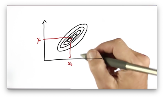
The mean of this Gaussian is the $(x_0, y_0)$ pair. The covariance defines the "spread" of the Gaussian as indicated by the contour lines.

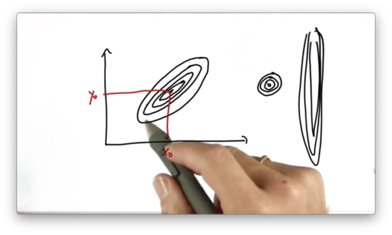
A two-dimensional Gaussian with a fairly small uncertainty would have much more tightly packed contour lines. Additionally, a 2D Gaussian might be very certain in one dimension and very uncertain in another. Both types are shown below.

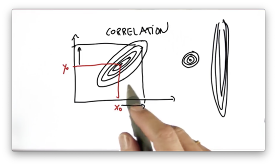
When the Gaussian is "tilted", as shown in the original graph, then $x$ and $y$ are correlated, which means that if we get information about the true value of $x$, we can make a corresponding inference about the true value of $y$.

For example, if we learn that the true value of $x_0$ is to the right of where we initially thought, we can adjust our estimate of $y_0$ a similar distance upwards.

Kalman Filter Prediction Quiz

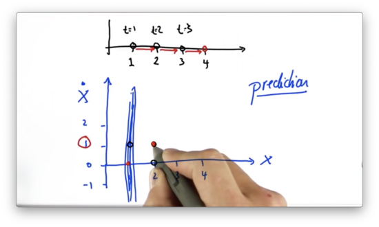
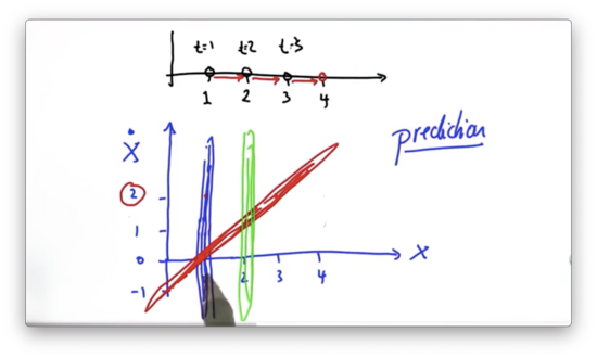
Let's look at a simple one-dimensional motion example. Assume we observe the following positions at the following timestamps.

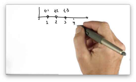
Given this information, we assume that, at time $t=4$, the object sits at position $x=4$. Even though we can only see the object's discrete locations, we can infer a velocity driving the object to the right. How does a Kalman filter address this?

Let's build a two-dimensional estimate, where one dimension corresponds to the position of the object, and the other dimension corresponds to the velocity of the object, denoted $\dot{x}$, which can be either negative, zero, or positive.

Initially, We know our location but not our velocity. We can represent this belief with a Gaussian that is narrow along the positional axis and elongated along the velocity axis.

Now let's look at the prediction step. Since we have a very low certainty for our velocity estimate, we cannot use it to predict a new position accurately.

Let's pause for a second and just assume a value for velocity: $\dot{x} = 0$. Given this assumption, along with the knowledge of the current position, $x = 0$, our prediction is the point $(0, 0)$, corresponding to a new position of 0 and a new velocity of 0. In other words, if we start somewhere and don't move, we can predict that we end up where we started.

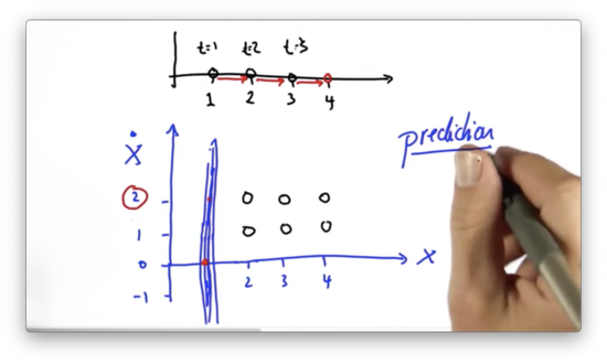
If we assume instead that the velocity $\dot{x} = 1$, where would the prediction be one time step later, given that we start at position $x = 1$?

Kalman Filter Prediction Quiz Solution

If we start with a velocity, $\dot{x} = 1$ and position, $x = 1$, then one time step in the future we predict our position to be updated by our velocity - $x = x + \dot{x} = 1 + 1 = 2$ - and our velocity to remain unchanged. This prediction corresponds with the point, $(2, 1)$.

Another Prediction Quiz

If we assume instead that the velocity $\dot{x} = 2$, which of the following points corresponds to the most plausible prediction one time step later, given that we start at position $x = 1$?

Another Prediction Quiz Solution

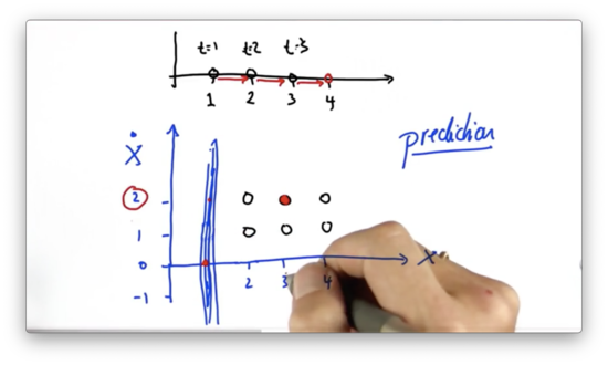
If we start with a velocity, $\dot{x} = 2$ and position, $x = 1$, then one time step in the future we predict our position to be updated by our velocity - $x = x + \dot{x} = 1 + 2 = 3$ - and our velocity to remain unchanged. This prediction corresponds with the point, $(3, 1)$.

More Kalman Filters

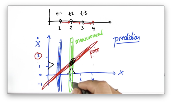
After we take our initial measurement, $x = 0$, we represent our current belief about our position and velocity with a Gaussian that is skinny along the position axis and elongated along the velocity axis.

The skinniness about the position axis indicates our relative certainty about our current position, while the elongation about the velocity axis indicates our total uncertainty about our current velocity.

Even though we are completely uncertain about our current velocity, we do know that our location and velocity are correlated. For example, given an initial measurement, $x = 0$, we expect to see a subsequent measurement, $x = 1$, if our velocity $\dot{x} = 1$. If our velocity $\dot{x} = 2$, we expect a subsequent measurement $x = 3$.

Given our initial measurement, we can generate a prediction Gaussian that essentially hugs the line mapping all possible subsequent positions to the velocities that would put us in those positions.

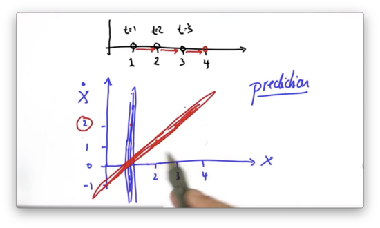
Even though we still haven't figured out how fast we are moving, we have pinned down the relationship between our position and our velocity, and we can illuminate the value of the latter by taking more measurements of the former.

Let's now fold in a second observation, $x = 2$, at time $t = 2$. Again, this observation tells us nothing about the velocity - only something about the location - which we can represent with the Gaussian in green below.

If we multiply the prior from the prediction step (in red above), with this measurement probability (green), then we get a Gaussian centered right about the point $(2,1)$. This Gaussian represents our current belief that our position $x = 2$ and our velocity $\dot{x} = 1$.

If we take this posterior Gaussian, in black above, and predict one step forward, we see a new Gaussian, centered at $(3,1)$, which corresponds to applying a constant velocity $\dot{x} = 1$ to a position $x = 2$.

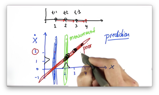
Note: This graphic is wrong. It represents increasing velocity: acceleration. All of the posterior distributions, shown in black, should be centered around $(x, 1)$. Read note here.

What's so powerful about this process is that we've been able to infer the value of a variable we couldn't directly measure using a variable we could measure. This inference is made possible by a physical equation that relates $x^\prime$, $x$, and $\dot{x}$.

This equation has been able to propagate constraints from subsequent measurements back to this unobservable variable, $\dot{x}$, so that we can estimate it. In other words, this equation defines the relationship between position and velocity, and, given two consecutive positional measurements, allows us to pin down a value of velocity, even though we cannot measure it directly.

This is the big lesson that Kalman filters teach us. The variables of a Kalman filter, often called states because they reflect states of the physical world, are separated into two subsets: the observables, like momentary location, and the hidden, like velocity.

Because these two variables are correlated, subsequent observations of the observable variables give us information about the hidden variables so that we can estimate the values of those hidden variables. In our case, we can estimate how fast an object is moving from multiple observations of its location.

Kalman Filter Design

When we design a Kalman filter, we need two functions: a state transition function and a measurement function. Let's look at both of these in the context of our 1D motion example.

Our state transition provides the following update rule for $x$: $x^\prime = x + \dot{x}\Delta{t}$. This function signifies that the resulting position is the sum of the current position and the product of the current velocity and the time delta. Additionally, our state transition provides the following update rule for $\dot{x}$: $\dot{x}^\prime = \dot{x}$. In other words, our velocity is constant.

We can express these two update rules simultaneously using linear algebra.

Our measurement function only observes the current position and not the velocity, and so we represent it like this.

We refer to the state transition matrix as $F$ and the measurement function matrix as $H$.

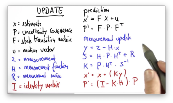
The actual update equations for Kalman filters, which generalize the specific example we have been using, are more involved.

In the prediction step, we update the current best estimate, $x$, by multiplying it with the state transition matrix, $F$, and adding the motion vector, $u$.

Our best estimate is accompanied by a covariance matrix, $P$, which characterizes the uncertainty of our estimate in each dimension of $x$. $P$ gets updated according to the following equation.

In the measurement update step, we first compute the error, $y$. This error is the difference between the measurement, $z$, and the product of the current estimate, $x$, and $H$, the matrix that maps the space of $x$ into the space of $z$.

The error is mapped into a matrix, $S$, which is obtained by projecting the system uncertainty, $P$, into the measurement space using the measurement function matrix, $H$, plus a matrix that characterizes the measurement noise, $R$.

We then compute a variable, $K$, which is often called the Kalman gain, where we invert $S$.

Finally, we update our estimate, $x$, and uncertainty, $P$, as follows.

Kalman Matrices Quiz

Let's complete one last challenging programming assignment. We are going to implement a multidimensional Kalman filter for the 1D motion/velocity example we have been investigating.

We are going to use a matrix class to help us manipulate matrices. This class can:

• initialize matrices from python lists
• zero out existing matrices
• compute an identity matrix
• print a matrix
• add, subtract, and multiply matrices
• compute the transpose of a matrix
• compute the inverse of a matrix

We can create a matrix like follows:

a = matrix([[10.], [10.]])

We can print the matrix with the show method:

a.show()
# [10.0]
# [10.0]

We can compute the transpose of a matrix using the transpose method:

b = a.transpose()
b.show()
# [10.0, 10.0]

We can multiply two matrices simply using the multiplication operator, which the matrix class overloads.

a = matrix([[10.], [10.]])
F = matrix([[12., 8.], [6., 2.]])
b = a * F
b.show()
# [200.0]
# [80.]

Using this library, let's set an initial state, x. This is a 1D tracking problem, so the state contains fields for the position and velocity.

x = matrix([[0.], [0.]])

We initialize an uncertainty matrix, p, which is characterized by a high uncertainty regarding both position and velocity.

P = matrix([[1000., 0.], [0., 1000.]])

We can specify an external motion u, but we set it to zero, so it has no effect.

u = matrix([[0.], [0.]])

We can specify the next state function, F, which takes on values according to the update rules we specified for each dimension in x.

F = matrix([[1., 1.], [0., 1.]])

We can specify a measurement function, H, which extracts the first of the two values. In other words, it observes the location but not the velocity.

H = matrix([[1., 0]])

We have a measurement uncertainty, R, which reflects the uncertainty in our positional measurements.

R = matrix([[1.]])

Finally, we have an identity matrix, I.

I = matrix([[1., 0.],[0., 1.]])

Additionally, we have a list of measurements, measurements = [1,2,3]. We want to implement a method, filter, which takes in the estimate, x, and uncertainty, P, and returns an estimate of velocity derived from those measurements.

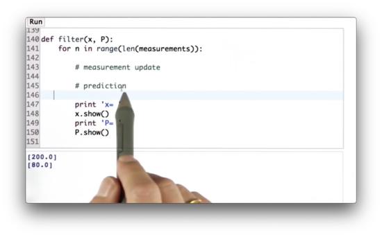
When implementing filter, we should program the measurement update first and then the motion update. Here is the shell of filter.

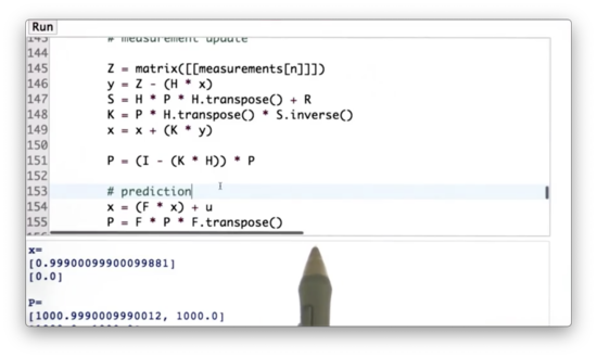
def filter(x, P):
    for n in range(len(measurements)):
        # measurement update
        # prediction
        print('x = ')
        x.show()
        print('P = ')
        P.show()

Once we run this function, we can see the following progress.

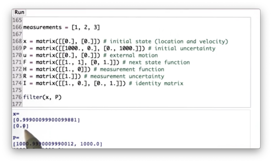
After the first measurement, we can see that we have essentially solved the localization problem, since x[0] correctly equals 1, but we haven't learned anything about velocity.

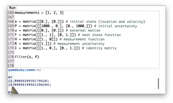
After the second run, we see that we have solved the localization problem and the velocity problem.

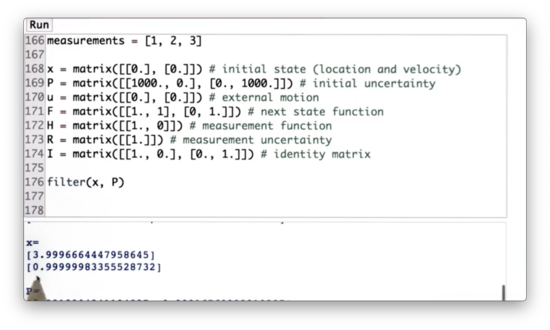
After the third measurement, we see that the estimate for both position and velocity remain correct.

Can you implement the method filter?

Kalman Matrices Quiz Solution

We can implement, in code, the measurement update and motion update rules we learned previously.

Note: We must convert the measurement into a matrix before subtracting H * x from it. Why? From the implementation of the overloaded multiplication operator (look for the __mul__ method, read more here), we see that the resulting product is an instance of the matrix class. As a result, if you try to compute measurements[n] - H * x, you will see the following error:

TypeError: unsupported operand type(s) for -: 'int' and 'instance'

Basically, you can't subtract an object from an integer. If you convert y into an instance of matrix - matrix([[y]]) - this error should go away.